 Catalog completeness#
This page shows how to use lfkit.LuminosityFunction to compute
observed and missing galaxy number densities for a magnitude-limited catalog.
Catalog completeness connects an apparent magnitude limit to the part of the luminosity function that is actually observable. At fixed survey depth, nearby galaxies can be observed to fainter intrinsic magnitudes, while at higher redshift only brighter galaxies remain above the catalog limit.
All examples below are executable via .. plot::.
The examples do not apply \(K\)-corrections or evolution corrections. Users
can pass correction values explicitly through the k_correction and
e_correction keyword arguments of the magnitude-limit and completeness
methods.
The number density units follow the normalization of the luminosity function. For example, if \(\phi_*\) is given in comoving \({\rm Mpc}^{-3}\), then the integrated number densities are also in \({\rm Mpc}^{-3}\). Fractions are dimensionless and are always defined relative to the chosen intrinsic absolute magnitude range.
Setup#
First define a cosmology and a luminosity function.
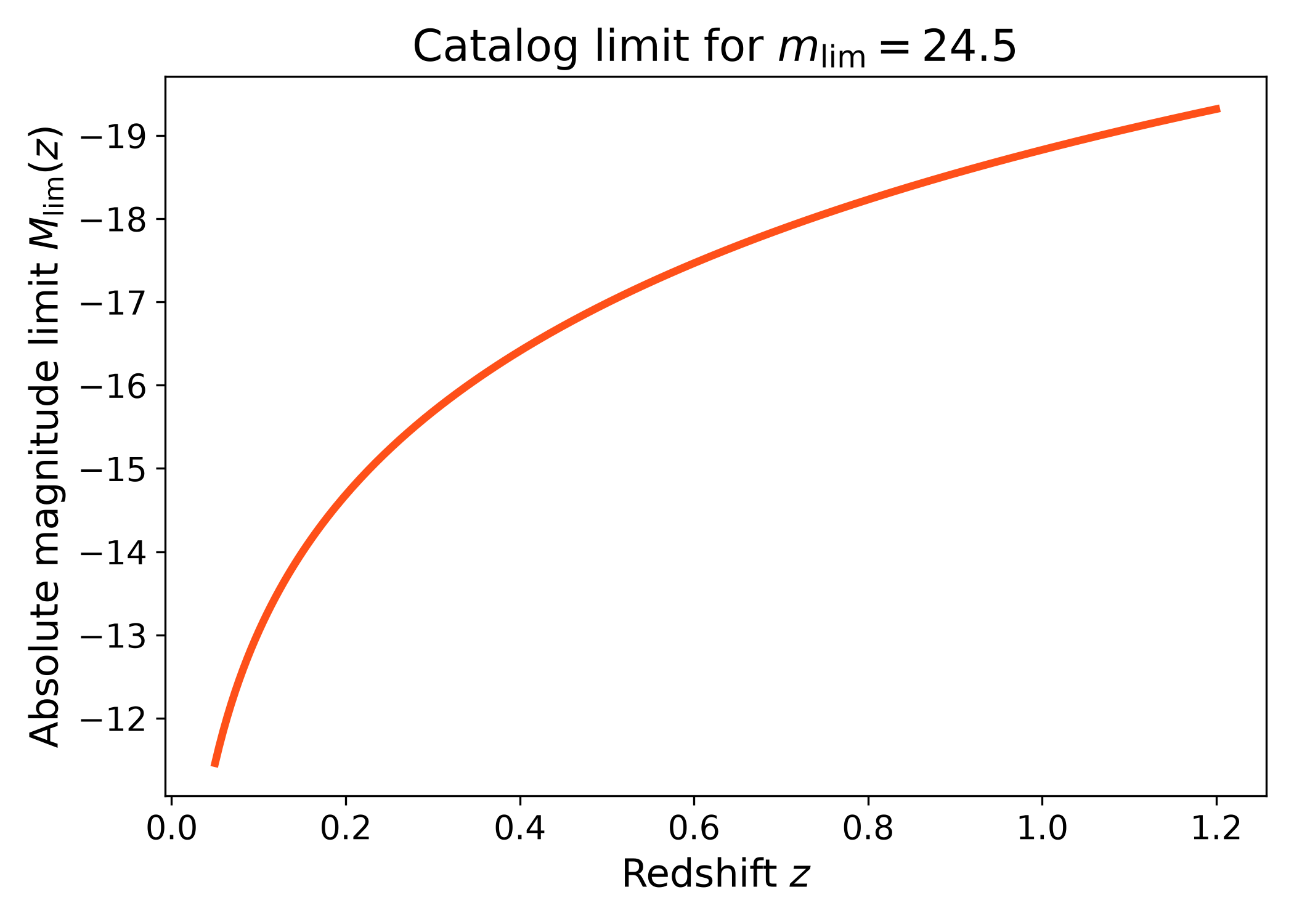
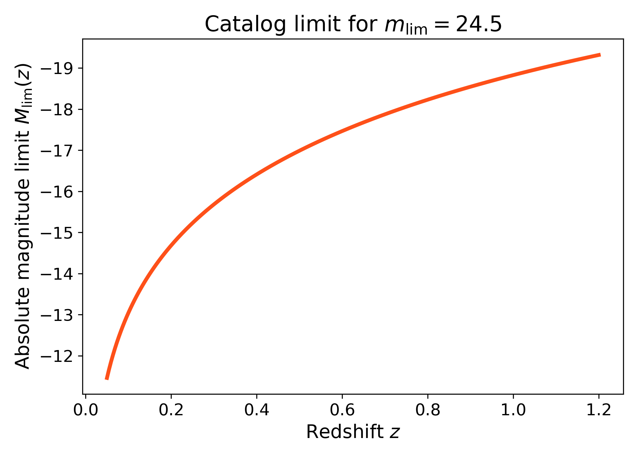
This setup plot shows the absolute magnitude limit implied by a fixed apparent magnitude cut. The curve answers a simple question: at each redshift, how bright does a galaxy need to be in absolute magnitude in order to enter the catalog?
The limit becomes brighter at higher redshift because distant galaxies must be intrinsically more luminous to remain above the same apparent magnitude threshold. The y-axis is inverted so that brighter absolute magnitudes appear higher on the plot.
import numpy as np
import matplotlib.pyplot as plt
import cmasher as cmr
import pyccl as ccl

from lfkit import LuminosityFunction

LABEL_SIZE = 15
TICK_SIZE = 13
TITLE_SIZE = 17
LEGEND_SIZE = 15

red = cmr.take_cmap_colors("cmr.guppy", 3, cmap_range=(0.0, 0.2))[1]

cosmo = ccl.Cosmology(
    Omega_c=0.25,
    Omega_b=0.05,
    h=0.7,
    sigma8=0.8,
    n_s=0.96,
    transfer_function="bbks",
    matter_power_spectrum="linear",
)

z = np.linspace(0.05, 1.2, 250)

lf = LuminosityFunction.evolving_schechter(
    phi_model="linear_p",
    phi_kwargs={"phi_0_star": 1.0e-3, "p": 0.8},
    m_star_model="linear_q",
    m_star_kwargs={"m_0_star": -20.5, "q": 1.0, "z_ref": 0.1},
    alpha_model="constant",
    alpha_kwargs={"alpha": -1.1},
)

m_limit = lf.completeness.absolute_magnitude_limit(
    cosmo,
    z,
    m_lim=24.5,
)

fig, ax = plt.subplots(figsize=(7.0, 5.0))
ax.plot(z, m_limit, lw=3, color=red)
ax.invert_yaxis()
ax.set_xlabel("Redshift $z$", fontsize=LABEL_SIZE)
ax.set_ylabel(r"Absolute magnitude limit $M_{\rm lim}(z)$", fontsize=LABEL_SIZE)
ax.set_title(r"Catalog limit for $m_{\rm lim}=24.5$", fontsize=TITLE_SIZE)
ax.tick_params(axis="both", labelsize=TICK_SIZE)
plt.tight_layout()
(png)
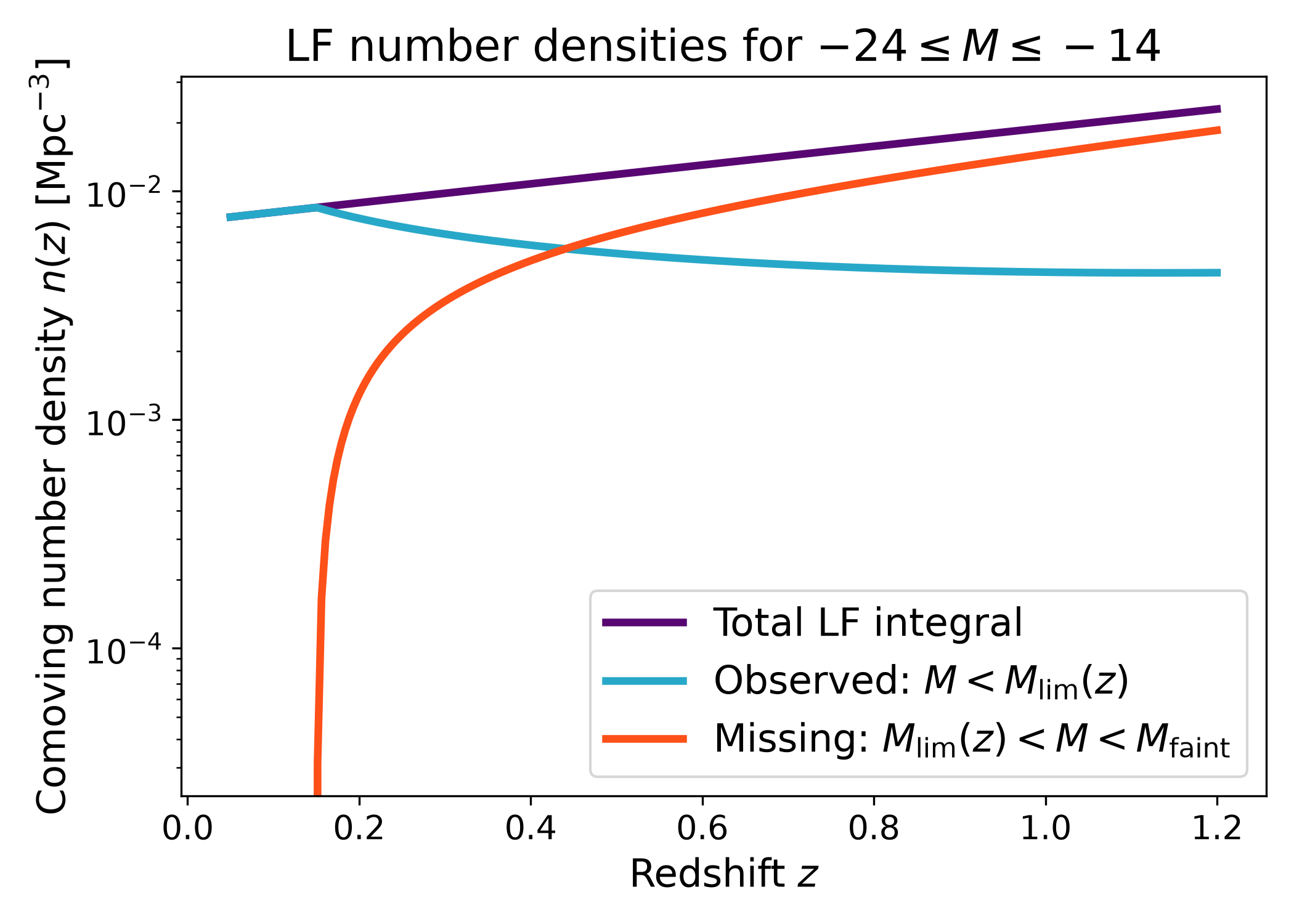
Observed and missing number densities#
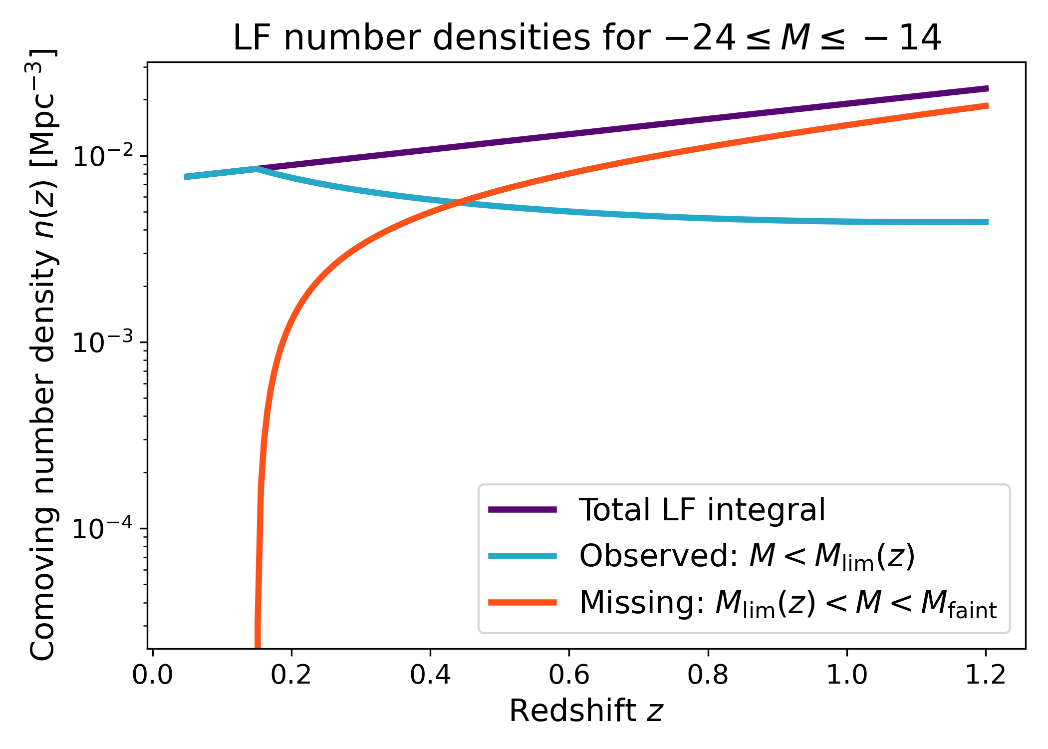
The observed number density is the part of the luminosity function brighter than the catalog limit. The missing number density is the part fainter than the catalog limit but still inside the requested absolute magnitude range.
This plot separates the full luminosity function integral into the part that is included in the catalog and the part that falls below the magnitude limit. At low redshift, the catalog limit is faint enough that most of the requested magnitude range can be observed. At higher redshift, the observed contribution shrinks and the missing contribution becomes more important.
This is useful when diagnosing whether a catalog is tracing most of the galaxy population described by the luminosity function, or only the bright tail of it.
import numpy as np
import matplotlib.pyplot as plt
import cmasher as cmr
import pyccl as ccl

from lfkit import LuminosityFunction

LABEL_SIZE = 15
TICK_SIZE = 13
TITLE_SIZE = 17
LEGEND_SIZE = 15

c_red = cmr.take_cmap_colors("cmr.guppy", 3, cmap_range=(0.0, 0.2))[1]
c_blue = cmr.take_cmap_colors("cmr.guppy", 3, cmap_range=(0.8, 1.0))[1]
c_mid = cmr.take_cmap_colors("cmr.guppy", 3, cmap_range=(0.0, 1.0))[1]

cosmo = ccl.Cosmology(
    Omega_c=0.25,
    Omega_b=0.05,
    h=0.7,
    sigma8=0.8,
    n_s=0.96,
    transfer_function="bbks",
    matter_power_spectrum="linear",
)

z = np.linspace(0.05, 1.2, 250)

lf = LuminosityFunction.evolving_schechter(
    phi_model="linear_p",
    phi_kwargs={"phi_0_star": 1.0e-3, "p": 0.8},
    m_star_model="linear_q",
    m_star_kwargs={"m_0_star": -20.5, "q": 1.0, "z_ref": 0.1},
    alpha_model="constant",
    alpha_kwargs={"alpha": -1.1},
)

m_bright = -24.0
m_faint = -14.0

n_total = lf.integrals.number_density(
    z,
    m_bright=m_bright,
    m_faint=m_faint,
)

n_obs = lf.completeness.observed_number_density(
    cosmo,
    z,
    m_lim=24.5,
    m_bright=m_bright,
    m_faint=m_faint,
)

n_miss = lf.completeness.missing_number_density(
    cosmo,
    z,
    m_lim=24.5,
    m_bright=m_bright,
    m_faint=m_faint,
)

fig, ax = plt.subplots(figsize=(7.0, 5.0))
ax.plot(z, n_total, lw=3, color=c_mid, label="Total LF integral")
ax.plot(z, n_obs, lw=3, color=c_blue, label=r"Observed: $M < M_{\rm lim}(z)$")
ax.plot(z, n_miss, lw=3, color=c_red, label=r"Missing: $M_{\rm lim}(z) < M < M_{\rm faint}$")
ax.set_yscale("log")
ax.set_xlabel("Redshift $z$", fontsize=LABEL_SIZE)
ax.set_ylabel(r"Comoving number density $n(z)$ [$\mathrm{Mpc}^{-3}$]", fontsize=LABEL_SIZE)
ax.set_title(r"LF number densities for $-24 \leq M \leq -14$", fontsize=TITLE_SIZE)
ax.tick_params(axis="both", labelsize=TICK_SIZE)
ax.legend(frameon=True, fontsize=LEGEND_SIZE, loc="best")
plt.tight_layout()
(png)
Completeness fraction#
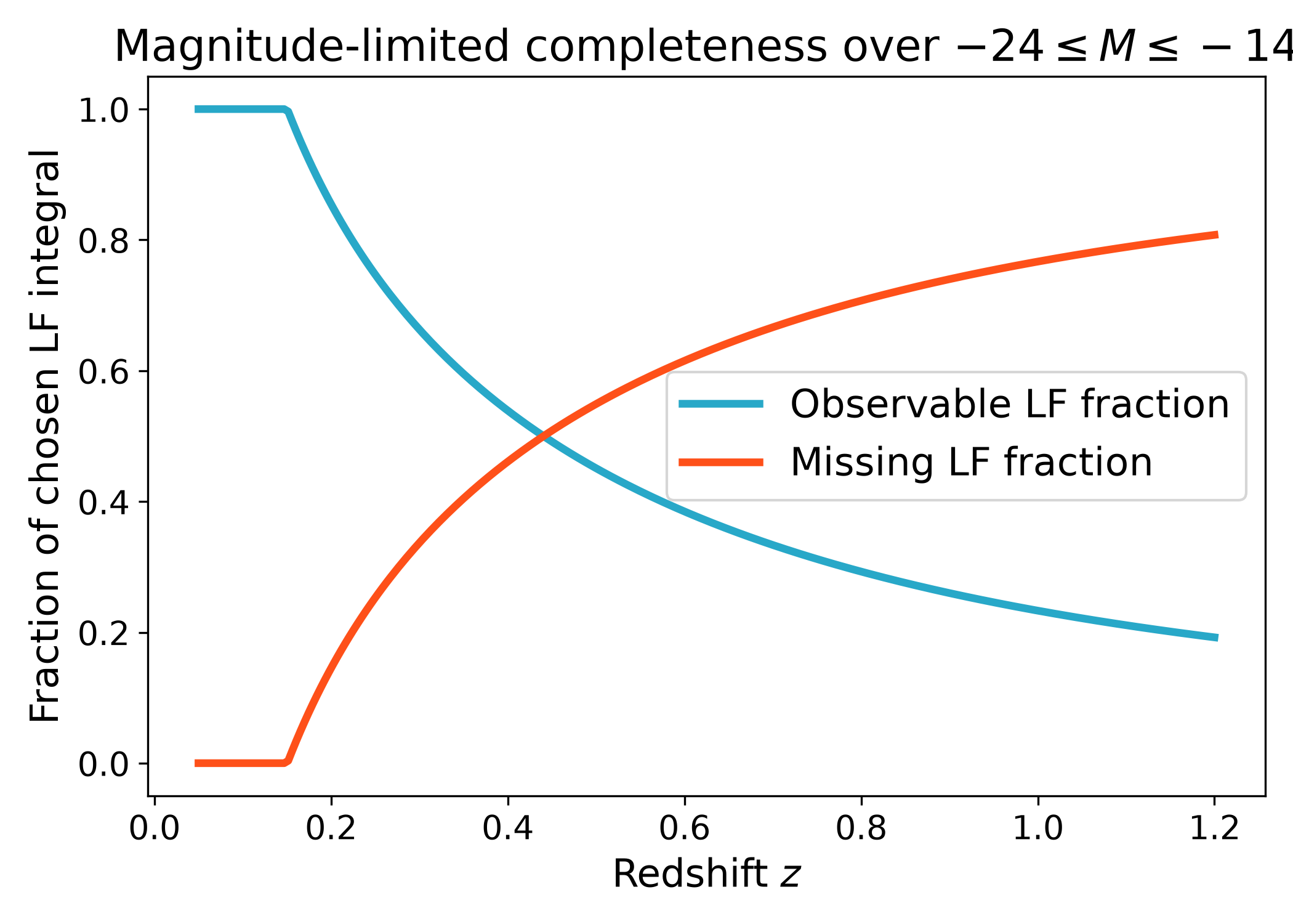
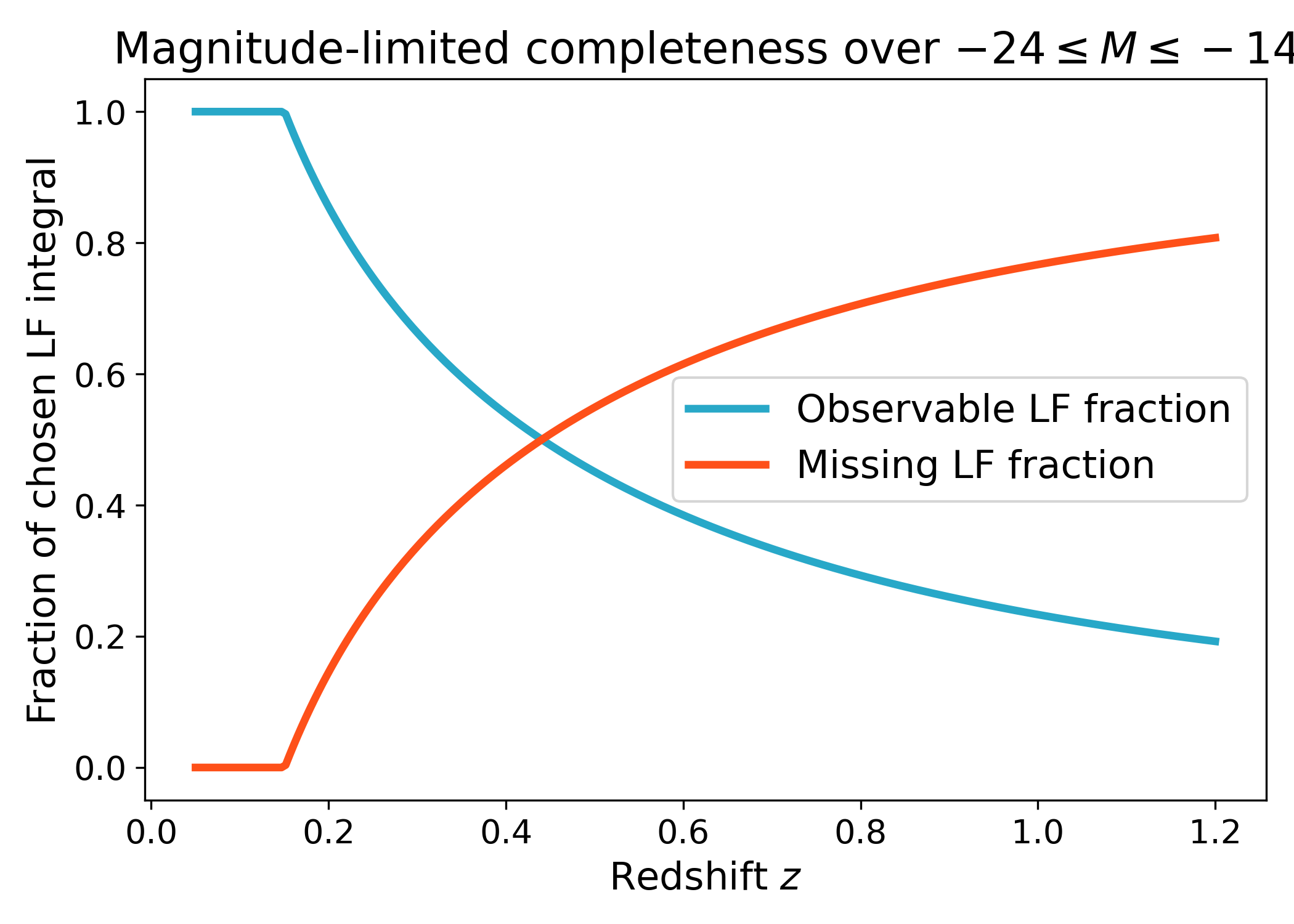
The catalog completeness fraction is the observed fraction of the integrated luminosity function over the chosen intrinsic absolute magnitude range.
This plot shows the same information as a fraction rather than as an absolute number density. The observed and missing fractions add up to one, so the figure directly shows how much of the requested luminosity function range is retained by the catalog limit.
This is often the most useful summary diagnostic. It tells you where the sample is effectively complete, where it is partially incomplete, and where the catalog contains only a small fraction of the intrinsic galaxy population.
import numpy as np
import matplotlib.pyplot as plt
import cmasher as cmr
import pyccl as ccl

from lfkit import LuminosityFunction

LABEL_SIZE = 15
TICK_SIZE = 13
TITLE_SIZE = 17
LEGEND_SIZE = 15

red = cmr.take_cmap_colors("cmr.guppy", 3, cmap_range=(0.0, 0.2))[1]
blue = cmr.take_cmap_colors("cmr.guppy", 3, cmap_range=(0.8, 1.0))[1]

cosmo = ccl.Cosmology(
    Omega_c=0.25,
    Omega_b=0.05,
    h=0.7,
    sigma8=0.8,
    n_s=0.96,
    transfer_function="bbks",
    matter_power_spectrum="linear",
)

z = np.linspace(0.05, 1.2, 250)

lf = LuminosityFunction.evolving_schechter(
    phi_model="linear_p",
    phi_kwargs={"phi_0_star": 1.0e-3, "p": 0.8},
    m_star_model="linear_q",
    m_star_kwargs={"m_0_star": -20.5, "q": 1.0, "z_ref": 0.1},
    alpha_model="constant",
    alpha_kwargs={"alpha": -1.1},
)

m_bright = -24.0
m_faint = -14.0

f_obs = lf.completeness.catalog_fraction(
    cosmo,
    z,
    m_lim=24.5,
    m_bright=m_bright,
    m_faint=m_faint,
)

f_miss = lf.completeness.out_of_catalog_fraction(
    cosmo,
    z,
    m_lim=24.5,
    m_bright=m_bright,
    m_faint=m_faint,
)

fig, ax = plt.subplots(figsize=(7.0, 5.0))
ax.plot(z, f_obs, lw=3, color=blue, label="Observable LF fraction")
ax.plot(z, f_miss, lw=3, color=red, label="Missing LF fraction")
ax.set_ylim(-0.05, 1.05)
ax.set_xlabel("Redshift $z$", fontsize=LABEL_SIZE)
ax.set_ylabel("Fraction of chosen LF integral", fontsize=LABEL_SIZE)
ax.set_title(r"Magnitude-limited completeness over $-24 \leq M \leq -14$", fontsize=TITLE_SIZE)
ax.tick_params(axis="both", labelsize=TICK_SIZE)
ax.legend(frameon=True, fontsize=LEGEND_SIZE, loc="center right")
plt.tight_layout()
(png)
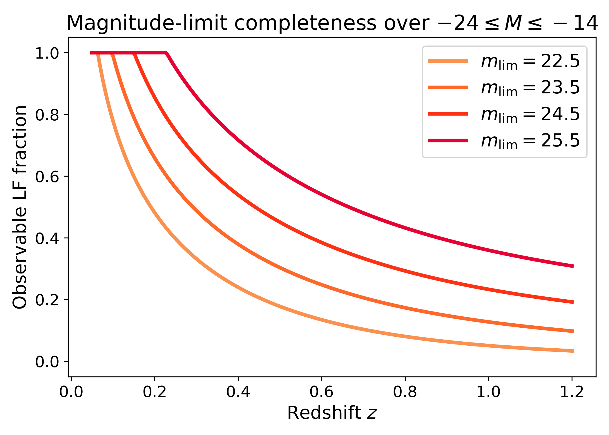
Comparing magnitude limits#
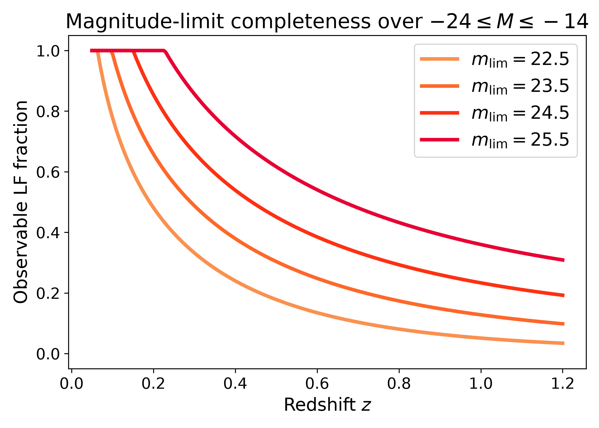
A fainter apparent magnitude limit observes a larger fraction of the luminosity function.
This plot compares catalog completeness for several survey depths. Shallower limits lose completeness earlier with redshift, while deeper limits retain a larger fraction of the luminosity function over a wider redshift range.
This is a useful way to visualize the gain from survey depth. A small change in the apparent magnitude limit can produce a large change in completeness, especially where the catalog is close to the transition between complete and incomplete.
import numpy as np
import matplotlib.pyplot as plt
import cmasher as cmr
import pyccl as ccl

from lfkit import LuminosityFunction

LABEL_SIZE = 15
TICK_SIZE = 13
TITLE_SIZE = 17
LEGEND_SIZE = 15

cosmo = ccl.Cosmology(
    Omega_c=0.25,
    Omega_b=0.05,
    h=0.7,
    sigma8=0.8,
    n_s=0.96,
    transfer_function="bbks",
    matter_power_spectrum="linear",
)

z = np.linspace(0.05, 1.2, 250)

lf = LuminosityFunction.evolving_schechter(
    phi_model="linear_p",
    phi_kwargs={"phi_0_star": 1.0e-3, "p": 0.8},
    m_star_model="linear_q",
    m_star_kwargs={"m_0_star": -20.5, "q": 1.0, "z_ref": 0.1},
    alpha_model="constant",
    alpha_kwargs={"alpha": -1.1},
)

limits = [22.5, 23.5, 24.5, 25.5]
colors = cmr.take_cmap_colors(
    "cmr.guppy",
    len(limits),
    cmap_range=(0.0, 0.2),
)

fig, ax = plt.subplots(figsize=(7.0, 5.0))

for m_lim, color in zip(limits, colors):
    f_obs = lf.completeness.catalog_fraction(
        cosmo,
        z,
        m_lim=m_lim,
        m_bright=-24.0,
        m_faint=-14.0,
    )
    ax.plot(z, f_obs, lw=3, color=color, label=rf"$m_{{\rm lim}}={m_lim}$")

ax.set_ylim(-0.05, 1.05)
ax.set_xlabel("Redshift $z$", fontsize=LABEL_SIZE)
ax.set_ylabel("Observable LF fraction", fontsize=LABEL_SIZE)
ax.set_title(r"Magnitude-limit completeness over $-24 \leq M \leq -14$", fontsize=TITLE_SIZE)
ax.tick_params(axis="both", labelsize=TICK_SIZE)
ax.legend(frameon=True, fontsize=LEGEND_SIZE, loc="best")
plt.tight_layout()
(png)
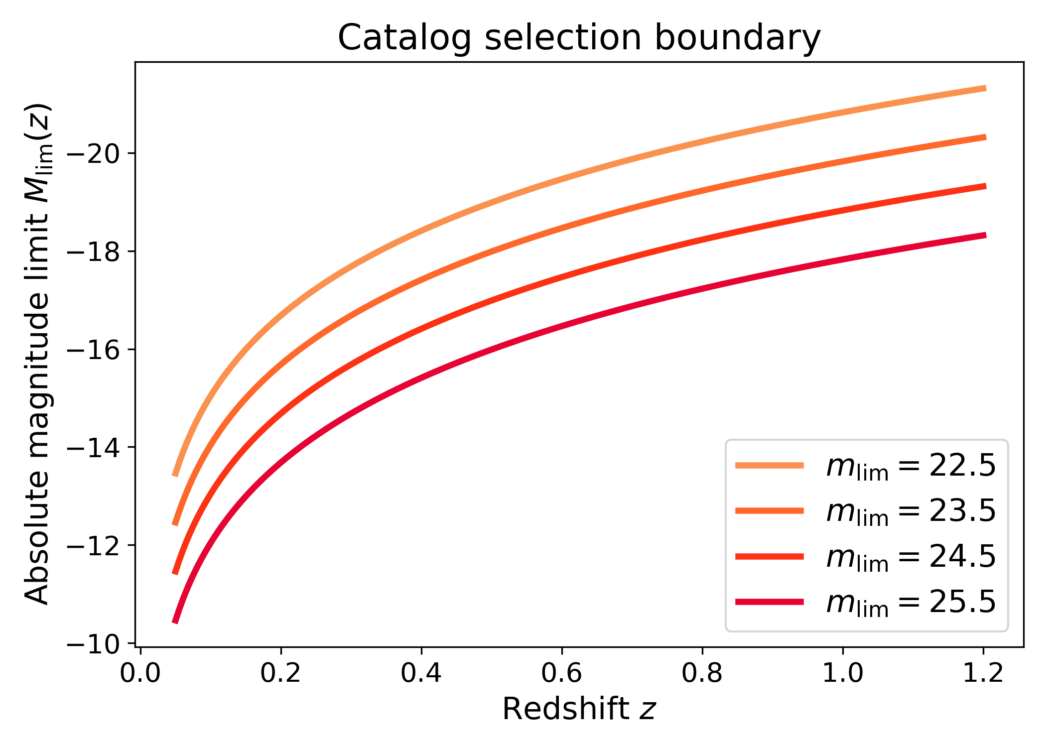
Absolute magnitude limits for different depths#
The apparent magnitude limit can also be shown directly as an absolute magnitude limit for several survey depths.
This plot shows how the catalog threshold moves in intrinsic luminosity as the survey becomes shallower or deeper. Deeper catalogs reach fainter absolute magnitudes at the same redshift, while shallower catalogs only include brighter galaxies.
This is a useful diagnostic before looking at completeness fractions, because it shows the selection boundary itself. The completeness calculation then asks how much of the luminosity function lies on the observable side of this boundary.
import numpy as np
import matplotlib.pyplot as plt
import cmasher as cmr
import pyccl as ccl

from lfkit import LuminosityFunction

LABEL_SIZE = 15
TICK_SIZE = 13
TITLE_SIZE = 17
LEGEND_SIZE = 15

cosmo = ccl.Cosmology(
    Omega_c=0.25,
    Omega_b=0.05,
    h=0.7,
    sigma8=0.8,
    n_s=0.96,
    transfer_function="bbks",
    matter_power_spectrum="linear",
)

z = np.linspace(0.05, 1.2, 250)

lf = LuminosityFunction.evolving_schechter(
    phi_model="linear_p",
    phi_kwargs={"phi_0_star": 1.0e-3, "p": 0.8},
    m_star_model="linear_q",
    m_star_kwargs={"m_0_star": -20.5, "q": 1.0, "z_ref": 0.1},
    alpha_model="constant",
    alpha_kwargs={"alpha": -1.1},
)

limits = [22.5, 23.5, 24.5, 25.5]
colors = cmr.take_cmap_colors(
    "cmr.guppy",
    len(limits),
    cmap_range=(0.0, 0.2),
)

fig, ax = plt.subplots(figsize=(7.0, 5.0))

for m_lim, color in zip(limits, colors):
    m_limit = lf.completeness.absolute_magnitude_limit(
        cosmo,
        z,
        m_lim=m_lim,
    )
    ax.plot(z, m_limit, lw=3, color=color, label=rf"$m_{{\rm lim}}={m_lim}$")

ax.invert_yaxis()
ax.set_xlabel("Redshift $z$", fontsize=LABEL_SIZE)
ax.set_ylabel(r"Absolute magnitude limit $M_{\rm lim}(z)$", fontsize=LABEL_SIZE)
ax.set_title("Catalog selection boundary", fontsize=TITLE_SIZE)
ax.tick_params(axis="both", labelsize=TICK_SIZE)
ax.legend(frameon=True, fontsize=LEGEND_SIZE, loc="best")
plt.tight_layout()
(png)
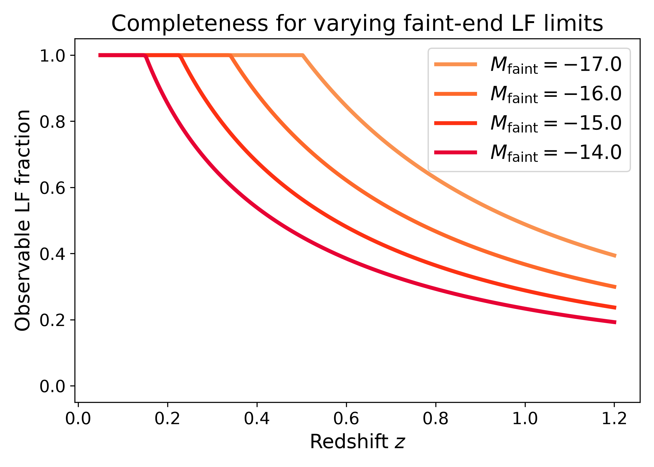
Dependence on the faint-end integration limit#
Completeness is always defined relative to a chosen intrinsic magnitude range.
This plot compares completeness fractions when the luminosity function is integrated down to different faint-end limits. Extending the intrinsic range to fainter galaxies usually lowers the completeness fraction, because the catalog must now account for a larger population of faint galaxies that may fall below the apparent magnitude limit.
This is an important sanity check. A catalog can appear highly complete if the requested intrinsic range is bright, but less complete if the calculation asks about a much fainter underlying population.
import numpy as np
import matplotlib.pyplot as plt
import cmasher as cmr
import pyccl as ccl

from lfkit import LuminosityFunction

LABEL_SIZE = 15
TICK_SIZE = 13
TITLE_SIZE = 17
LEGEND_SIZE = 15

cosmo = ccl.Cosmology(
    Omega_c=0.25,
    Omega_b=0.05,
    h=0.7,
    sigma8=0.8,
    n_s=0.96,
    transfer_function="bbks",
    matter_power_spectrum="linear",
)

z = np.linspace(0.05, 1.2, 250)

lf = LuminosityFunction.evolving_schechter(
    phi_model="linear_p",
    phi_kwargs={"phi_0_star": 1.0e-3, "p": 0.8},
    m_star_model="linear_q",
    m_star_kwargs={"m_0_star": -20.5, "q": 1.0, "z_ref": 0.1},
    alpha_model="constant",
    alpha_kwargs={"alpha": -1.1},
)

faint_limits = [-17.0, -16.0, -15.0, -14.0]
colors = cmr.take_cmap_colors(
    "cmr.guppy",
    len(faint_limits),
    cmap_range=(0.0, 0.2),
)

fig, ax = plt.subplots(figsize=(7.0, 5.0))

for m_faint, color in zip(faint_limits, colors):
    f_obs = lf.completeness.catalog_fraction(
        cosmo,
        z,
        m_lim=24.5,
        m_bright=-24.0,
        m_faint=m_faint,
    )
    ax.plot(
        z,
        f_obs,
        lw=3,
        color=color,
        label=rf"$M_{{\rm faint}}={m_faint}$",
    )

ax.set_ylim(-0.05, 1.05)
ax.set_xlabel("Redshift $z$", fontsize=LABEL_SIZE)
ax.set_ylabel("Observable LF fraction", fontsize=LABEL_SIZE)
ax.set_title(r"Completeness for varying faint-end LF limits", fontsize=TITLE_SIZE)
ax.tick_params(axis="both", labelsize=TICK_SIZE)
ax.legend(frameon=True, fontsize=LEGEND_SIZE, loc="best")
plt.tight_layout()
(png)

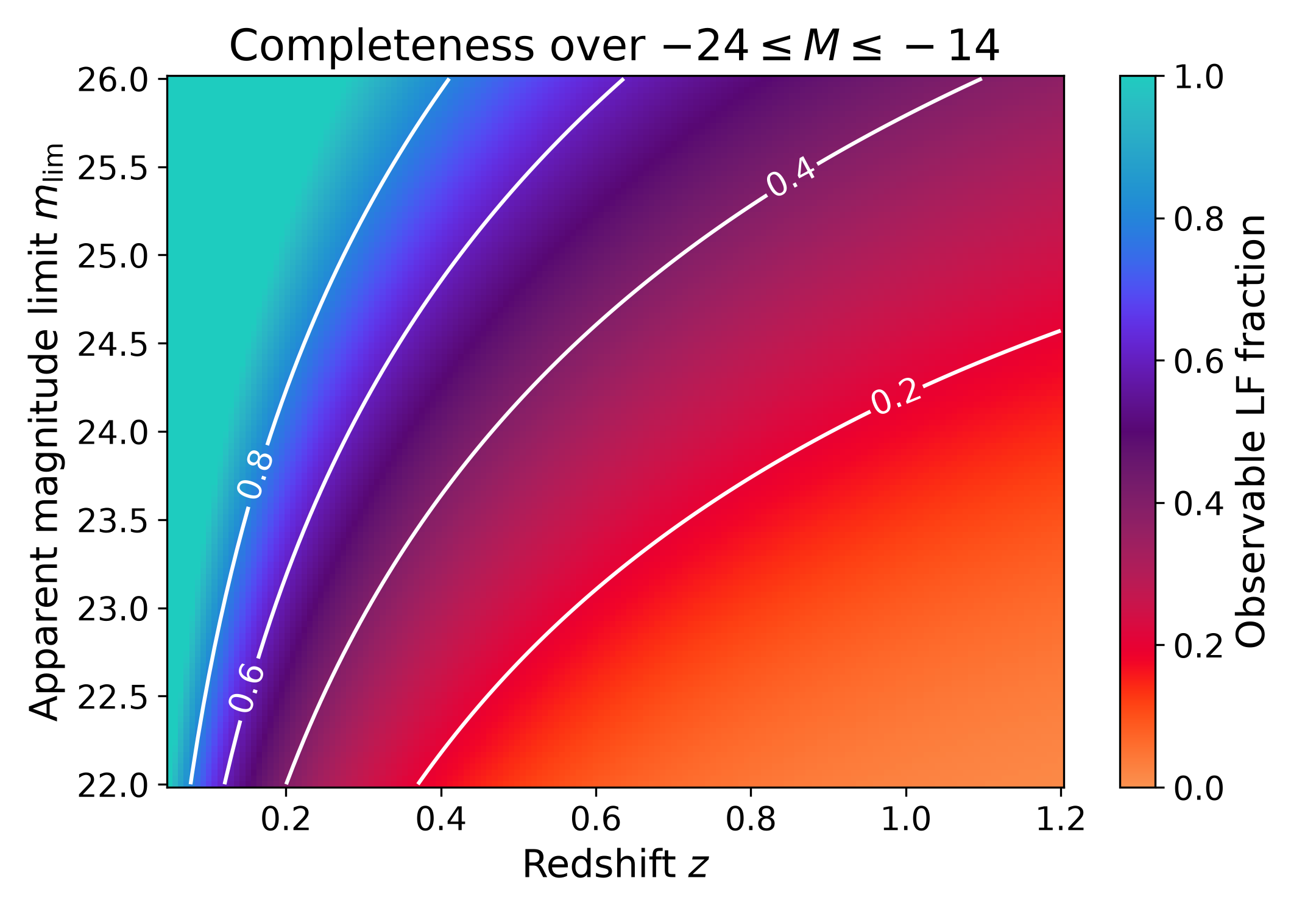
Completeness as a redshift-depth surface#
Completeness can also be viewed as a two-dimensional function of redshift and survey depth.
This plot shows how much of the chosen intrinsic galaxy population is visible for different combinations of redshift and apparent magnitude limit. The horizontal axis changes redshift, while the vertical axis changes catalog depth: larger \(m_{\rm lim}\) values correspond to deeper catalogs.
The colour scale gives the observable fraction of the luminosity function integral over \(-24 \leq M \leq -14\), after applying the apparent magnitude cut. A value near one means that almost all galaxies in this intrinsic magnitude range are included in the catalog. A value near zero means that only a small part of that population is bright enough to pass the apparent magnitude cut.
The white contours mark fixed observable LF fractions of 0.2, 0.4, 0.6, and 0.8. In plain terms, the 0.8 contour is the line where the catalog keeps about 80 per cent of the chosen luminosity function integral, while the 0.2 contour is where it keeps only about 20 per cent.
This kind of summary is helpful when choosing survey depths or checking which redshift range is safe for a magnitude-limited sample.
import numpy as np
import matplotlib.pyplot as plt
import cmasher as cmr
import pyccl as ccl

from lfkit import LuminosityFunction

LABEL_SIZE = 15
TICK_SIZE = 13
TITLE_SIZE = 17
LEGEND_SIZE = 15

cosmo = ccl.Cosmology(
    Omega_c=0.25,
    Omega_b=0.05,
    h=0.7,
    sigma8=0.8,
    n_s=0.96,
    transfer_function="bbks",
    matter_power_spectrum="linear",
)

z = np.linspace(0.05, 1.2, 160)
limits = np.linspace(22.0, 26.0, 120)

lf = LuminosityFunction.evolving_schechter(
    phi_model="linear_p",
    phi_kwargs={"phi_0_star": 1.0e-3, "p": 0.8},
    m_star_model="linear_q",
    m_star_kwargs={"m_0_star": -20.5, "q": 1.0, "z_ref": 0.1},
    alpha_model="constant",
    alpha_kwargs={"alpha": -1.1},
)

completeness = []

for m_lim in limits:
    f_obs = lf.completeness.catalog_fraction(
        cosmo,
        z,
        m_lim=m_lim,
        m_bright=-24.0,
        m_faint=-14.0,
    )
    completeness.append(f_obs)

completeness = np.asarray(completeness)

fig, ax = plt.subplots(figsize=(7.2, 5.0))

mesh = ax.pcolormesh(
    z,
    limits,
    completeness,
    shading="auto",
    cmap="cmr.guppy",
    vmin=0.0,
    vmax=1.0,
)

contour_levels = [0.2, 0.4, 0.6, 0.8]
contours = ax.contour(
    z,
    limits,
    completeness,
    levels=contour_levels,
    colors="white",
    linewidths=1.5,
)
ax.clabel(contours, inline=True, fontsize=TICK_SIZE, fmt="%.1f")

ax.set_xlabel("Redshift $z$", fontsize=LABEL_SIZE)
ax.set_ylabel(r"Apparent magnitude limit $m_{\rm lim}$", fontsize=LABEL_SIZE)
ax.set_title(r"Completeness over $-24 \leq M \leq -14$", fontsize=TITLE_SIZE)
ax.tick_params(axis="both", labelsize=TICK_SIZE)

cbar = fig.colorbar(mesh, ax=ax)
cbar.set_label(r"Observable LF fraction", fontsize=LABEL_SIZE)
cbar.ax.tick_params(labelsize=TICK_SIZE)

plt.tight_layout()
(png)

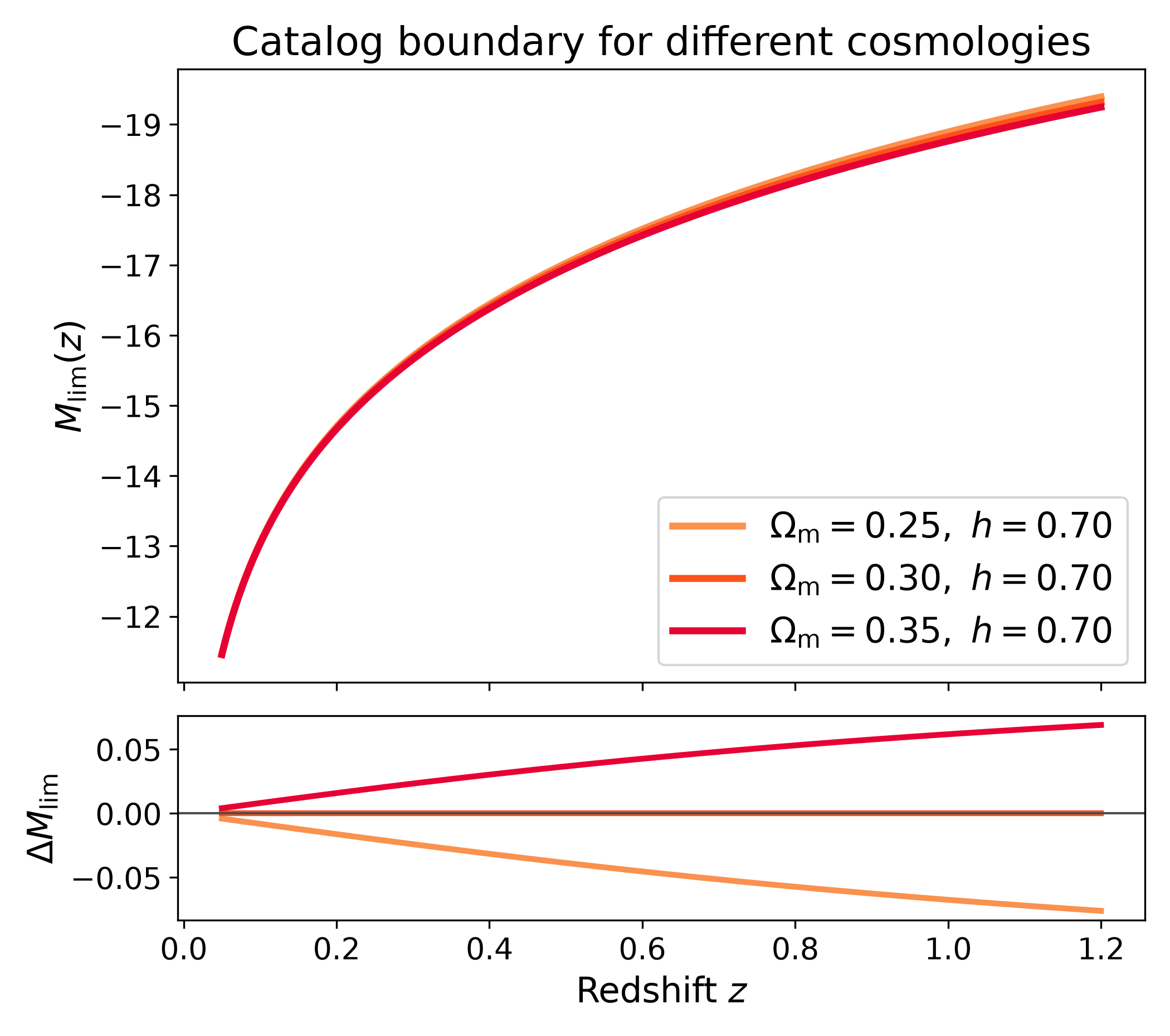
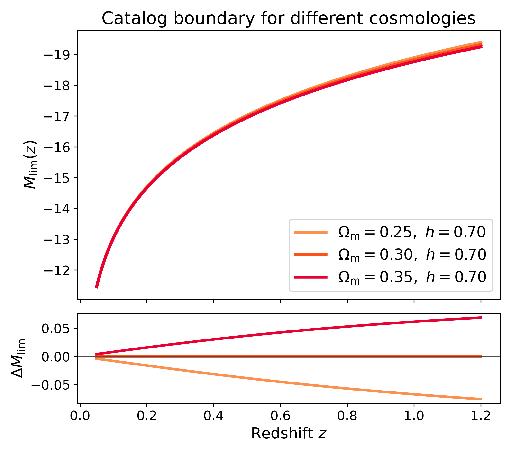
Comparing cosmologies#
The absolute magnitude limit depends on cosmology through the luminosity distance and distance modulus. This means that the same apparent magnitude limit can correspond to slightly different intrinsic magnitude cuts in different cosmologies.
The example below compares three cosmologies. The luminosity function is kept
fixed, so the plot isolates the effect of the cosmology-dependent magnitude
conversion. Users can replace the dictionary entries with any
pyccl.Cosmology objects relevant to their analysis.
The lower panel shows the residual relative to the reference cosmology, \(\Omega_{\rm m}=0.30,\ h=0.70\).
import numpy as np
import matplotlib.pyplot as plt
import cmasher as cmr
import pyccl as ccl

from lfkit import LuminosityFunction

LABEL_SIZE = 15
TICK_SIZE = 13
TITLE_SIZE = 17
LEGEND_SIZE = 15

cosmologies = {
    r"$\Omega_{\rm m}=0.25,\ h=0.70$": ccl.Cosmology(
        Omega_c=0.20,
        Omega_b=0.05,
        h=0.70,
        sigma8=0.8,
        n_s=0.96,
        transfer_function="bbks",
        matter_power_spectrum="linear",
    ),
    r"$\Omega_{\rm m}=0.30,\ h=0.70$": ccl.Cosmology(
        Omega_c=0.25,
        Omega_b=0.05,
        h=0.70,
        sigma8=0.8,
        n_s=0.96,
        transfer_function="bbks",
        matter_power_spectrum="linear",
    ),
    r"$\Omega_{\rm m}=0.35,\ h=0.70$": ccl.Cosmology(
        Omega_c=0.30,
        Omega_b=0.05,
        h=0.70,
        sigma8=0.8,
        n_s=0.96,
        transfer_function="bbks",
        matter_power_spectrum="linear",
    ),
}

z = np.linspace(0.05, 1.2, 250)

lf = LuminosityFunction.evolving_schechter(
    phi_model="linear_p",
    phi_kwargs={"phi_0_star": 1.0e-3, "p": 0.8},
    m_star_model="linear_q",
    m_star_kwargs={"m_0_star": -20.5, "q": 1.0, "z_ref": 0.1},
    alpha_model="constant",
    alpha_kwargs={"alpha": -1.1},
)

m_limits = {}

for label, cosmo in cosmologies.items():
    m_limits[label] = lf.completeness.absolute_magnitude_limit(
        cosmo,
        z,
        m_lim=24.5,
    )

reference_label = r"$\Omega_{\rm m}=0.30,\ h=0.70$"
reference = m_limits[reference_label]

colors = cmr.take_cmap_colors(
    "cmr.guppy",
    len(cosmologies),
    cmap_range=(0.0, 0.2),
)

fig, (ax_top, ax_bottom) = plt.subplots(
    2,
    1,
    figsize=(7.0, 6.2),
    sharex=True,
    gridspec_kw={"height_ratios": [3, 1]},
)

for (label, m_limit), color in zip(m_limits.items(), colors):
    ax_top.plot(z, m_limit, lw=3, color=color, label=label)
    ax_bottom.plot(z, m_limit - reference, lw=2.5, color=color)

ax_top.invert_yaxis()
ax_top.set_ylabel(r"$M_{\rm lim}(z)$", fontsize=LABEL_SIZE)
ax_top.set_title(r"Catalog boundary for different cosmologies", fontsize=TITLE_SIZE)
ax_top.legend(frameon=True, fontsize=LEGEND_SIZE, loc="best")

ax_bottom.axhline(0.0, lw=1.0, color="0.3")
ax_bottom.set_xlabel("Redshift $z$", fontsize=LABEL_SIZE)
ax_bottom.set_ylabel(r"$\Delta M_{\rm lim}$", fontsize=LABEL_SIZE)

for ax in (ax_top, ax_bottom):
    ax.tick_params(axis="both", labelsize=TICK_SIZE)

plt.tight_layout()
(png)
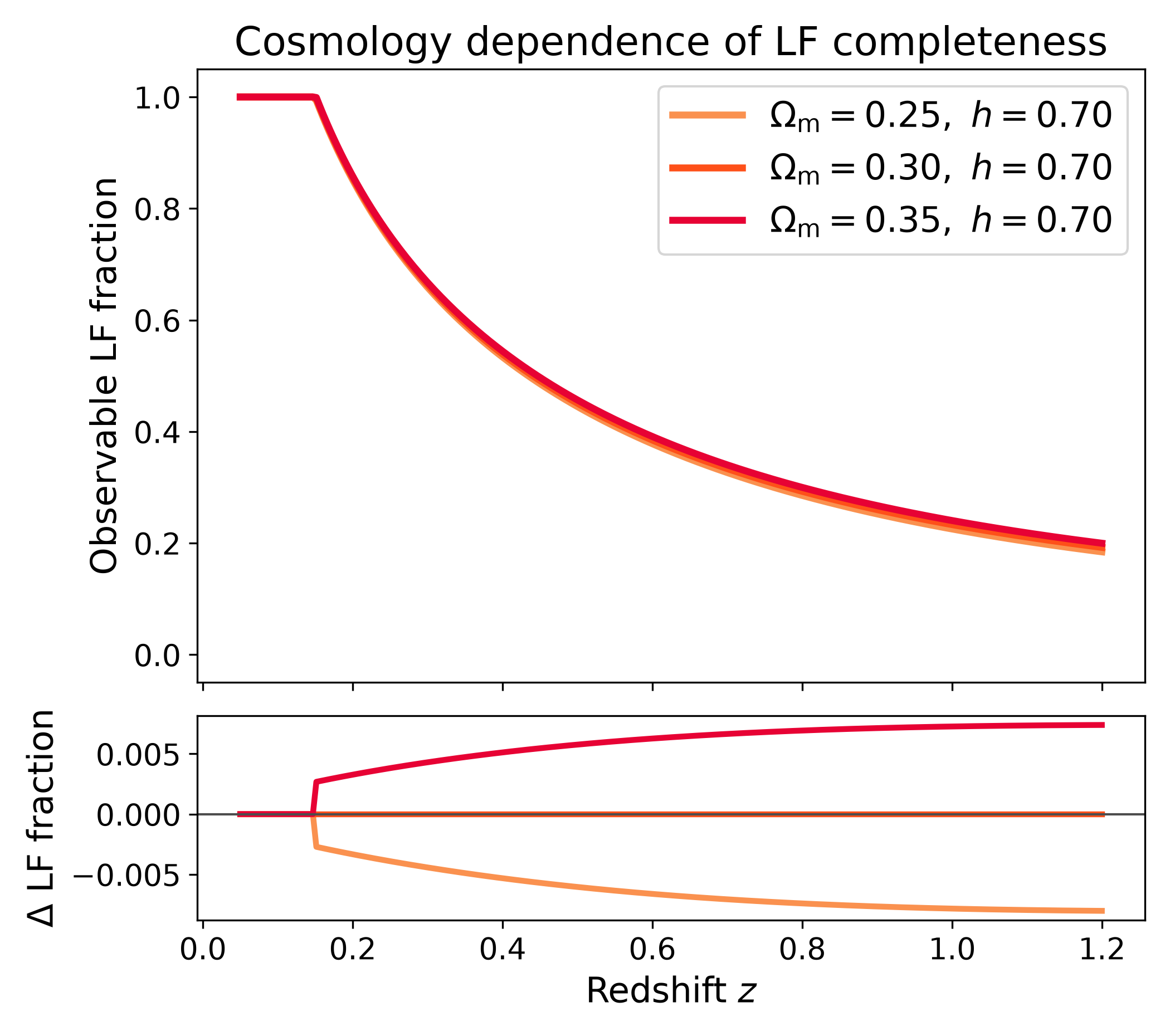
Completeness for different cosmologies#
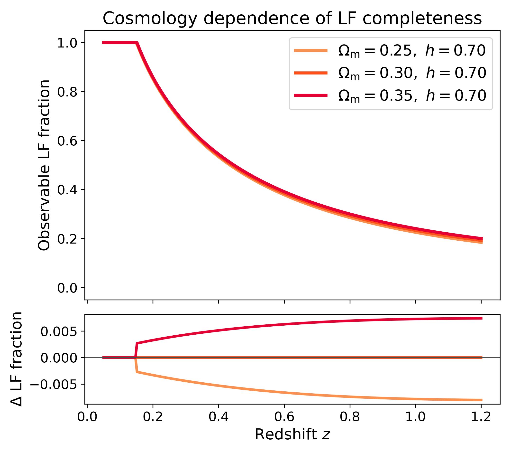
Changing cosmology also changes the completeness fraction through the cosmology-dependent apparent-to-absolute magnitude conversion.
This comparison keeps the luminosity function, apparent magnitude limit, and intrinsic magnitude range fixed. Only the cosmology is changed. This makes the plot useful for checking how sensitive the catalog-completeness calculation is to the assumed distance-redshift relation.
The lower panel shows the residual relative to the reference cosmology, \(\Omega_{\rm m}=0.30,\ h=0.70\).
import numpy as np
import matplotlib.pyplot as plt
import cmasher as cmr
import pyccl as ccl

from lfkit import LuminosityFunction

LABEL_SIZE = 15
TICK_SIZE = 13
TITLE_SIZE = 17
LEGEND_SIZE = 15

cosmologies = {
    r"$\Omega_{\rm m}=0.25,\ h=0.70$": ccl.Cosmology(
        Omega_c=0.20,
        Omega_b=0.05,
        h=0.70,
        sigma8=0.8,
        n_s=0.96,
        transfer_function="bbks",
        matter_power_spectrum="linear",
    ),
    r"$\Omega_{\rm m}=0.30,\ h=0.70$": ccl.Cosmology(
        Omega_c=0.25,
        Omega_b=0.05,
        h=0.70,
        sigma8=0.8,
        n_s=0.96,
        transfer_function="bbks",
        matter_power_spectrum="linear",
    ),
    r"$\Omega_{\rm m}=0.35,\ h=0.70$": ccl.Cosmology(
        Omega_c=0.30,
        Omega_b=0.05,
        h=0.70,
        sigma8=0.8,
        n_s=0.96,
        transfer_function="bbks",
        matter_power_spectrum="linear",
    ),
}

colors = cmr.take_cmap_colors(
    "cmr.guppy",
    len(cosmologies),
    cmap_range=(0.0, 0.2),
)

z = np.linspace(0.05, 1.2, 250)

lf = LuminosityFunction.evolving_schechter(
    phi_model="linear_p",
    phi_kwargs={"phi_0_star": 1.0e-3, "p": 0.8},
    m_star_model="linear_q",
    m_star_kwargs={"m_0_star": -20.5, "q": 1.0, "z_ref": 0.1},
    alpha_model="constant",
    alpha_kwargs={"alpha": -1.1},
)

completeness = {}

for label, cosmo in cosmologies.items():
    completeness[label] = lf.completeness.catalog_fraction(
        cosmo,
        z,
        m_lim=24.5,
        m_bright=-24.0,
        m_faint=-14.0,
    )

reference_label = r"$\Omega_{\rm m}=0.30,\ h=0.70$"
reference = completeness[reference_label]

fig, (ax_top, ax_bottom) = plt.subplots(
    2,
    1,
    figsize=(7.0, 6.2),
    sharex=True,
    gridspec_kw={"height_ratios": [3, 1]},
)

for (label, f_obs), color in zip(completeness.items(), colors):
    ax_top.plot(z, f_obs, lw=3, color=color, label=label)
    ax_bottom.plot(z, f_obs - reference, lw=2.5, color=color)

ax_top.set_ylim(-0.05, 1.05)
ax_top.set_ylabel("Observable LF fraction", fontsize=LABEL_SIZE)
ax_top.set_title(r"Cosmology dependence of LF completeness", fontsize=TITLE_SIZE)
ax_top.legend(frameon=True, fontsize=LEGEND_SIZE, loc="best")

ax_bottom.axhline(0.0, lw=1.0, color="0.3")
ax_bottom.set_xlabel("Redshift $z$", fontsize=LABEL_SIZE)
ax_bottom.set_ylabel(r"$\Delta$ LF fraction", fontsize=LABEL_SIZE)

for ax in (ax_top, ax_bottom):
    ax.tick_params(axis="both", labelsize=TICK_SIZE)

plt.tight_layout()
(png)