 Luminosity function models#
This page introduces the luminosity function models exposed by
lfkit.LuminosityFunction. These models describe the abundance of
galaxies as a function of magnitude, usually written as \(\Phi(M)\).
The examples focus on constructing, evaluating, visualizing, and comparing luminosity function models. Magnitude integrals, completeness calculations, apparent magnitude limits, redshift-density weighting, and conditional luminosity functions are covered on separate pages.
The API is centered on lfkit.LuminosityFunction. A luminosity function
object stores the chosen model and evaluates it through
lfkit.LuminosityFunction.phi().
The number-density units follow the normalization supplied to the luminosity
function. For example, if phi_star is supplied in
\({\rm Mpc}^{-3}\,{\rm mag}^{-1}\), then \(\Phi(M)\) has units of
\({\rm Mpc}^{-3}\,{\rm mag}^{-1}\).
Schechter family models#
The Schechter family is the main luminosity function model family currently exposed by LFKit. It includes the standard Schechter model, double-Schechter variants, and redshift-evolving Schechter models.
These models are useful for describing galaxy luminosity functions with a power-law faint end and an exponential bright-end cutoff. The faint end controls the abundance of low-luminosity galaxies, while the bright-end cutoff suppresses very luminous galaxies. The examples below show how to construct, evaluate, compare, and inspect Schechter-family models.
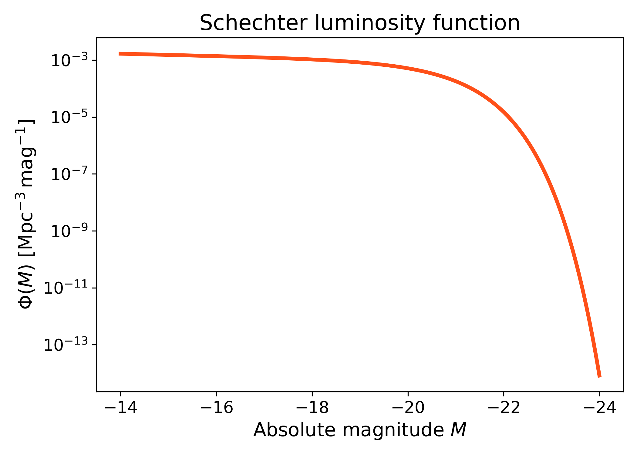
Standard Schechter luminosity function#
A Schechter luminosity function can be created with
lfkit.LuminosityFunction.schechter(). The returned object evaluates
\(\Phi(M)\) through lfkit.LuminosityFunction.phi().
This example shows the basic shape of the model in absolute magnitude. The curve rises toward fainter magnitudes because of the power-law faint end, while the abundance drops rapidly at the bright end because of the exponential cutoff.
import numpy as np
import matplotlib.pyplot as plt
import cmasher as cmr

from lfkit import LuminosityFunction

LABEL_SIZE = 15
TICK_SIZE = 13
TITLE_SIZE = 17

lf = LuminosityFunction.schechter(
    phi_star=1.0e-3,
    m_star=-20.5,
    alpha=-1.1,
)

absolute_mag = np.linspace(-24.0, -14.0, 500)
phi = lf.phi(absolute_mag)

fig, ax = plt.subplots(figsize=(7.0, 5.0))
ax.plot(
    absolute_mag,
    phi,
    lw=3,
    color=cmr.take_cmap_colors("cmr.guppy", 3, cmap_range=(0., 0.2))[1],
)

ax.set_yscale("log")
ax.invert_xaxis()
ax.set_xlabel("Absolute magnitude $M$", fontsize=LABEL_SIZE)
ax.set_ylabel(
    r"$\Phi(M)$ [$\mathrm{Mpc}^{-3}\,\mathrm{mag}^{-1}$]",
    fontsize=LABEL_SIZE,
)
ax.set_title("Schechter luminosity function", fontsize=TITLE_SIZE)
ax.tick_params(axis="both", labelsize=TICK_SIZE)
plt.tight_layout()
(png)

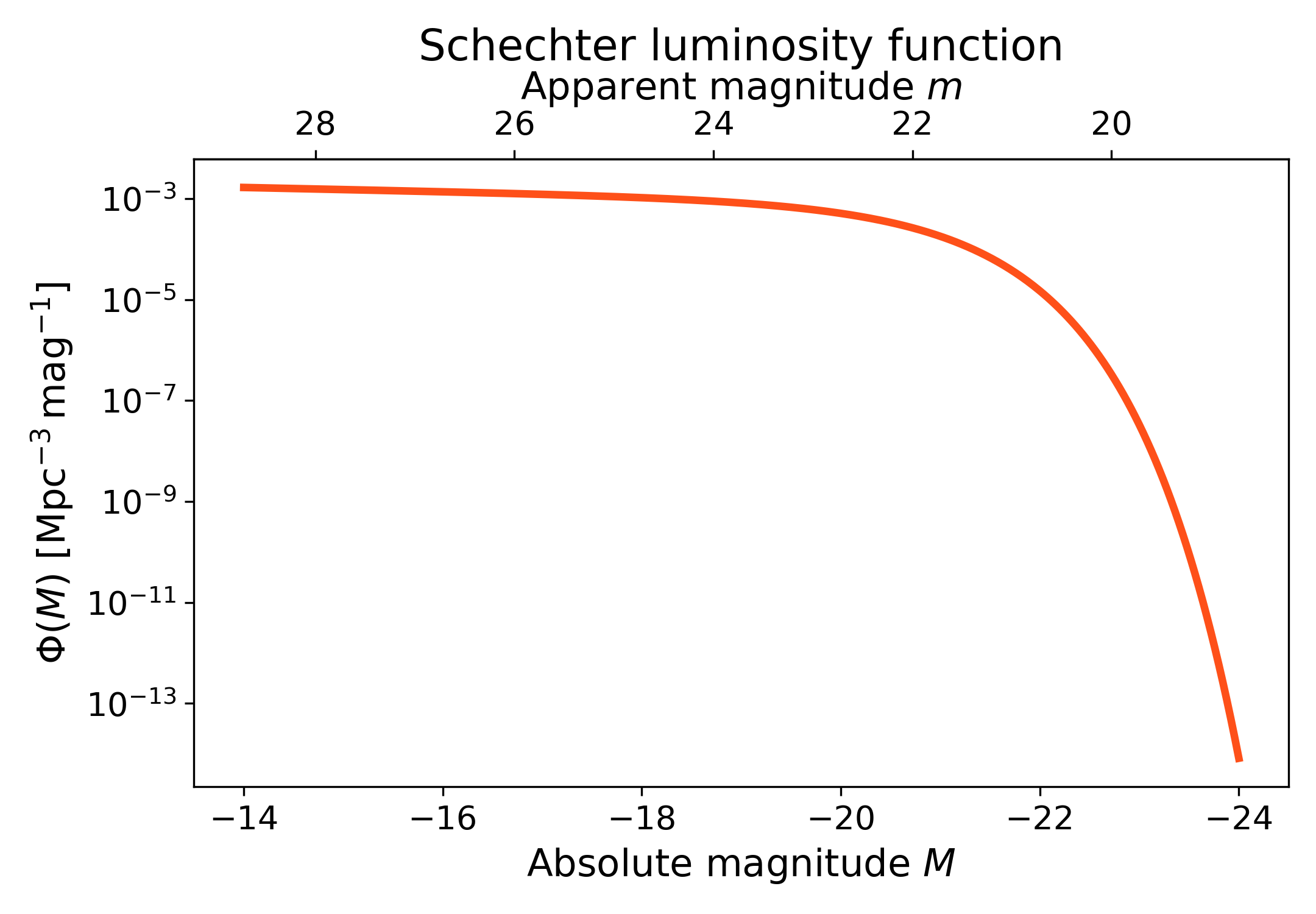
Standard Schechter luminosity function with apparent magnitude axis#
The Schechter luminosity function is evaluated in absolute magnitude. A secondary x-axis can show the corresponding apparent magnitude at a fixed luminosity distance using the LFKit magnitude converters.
This keeps the model-native absolute magnitude axis while also showing where the same magnitude range would appear observationally. The apparent magnitude axis is only a reference conversion for the chosen luminosity distance; changing that distance would shift the upper axis.
import numpy as np
import matplotlib.pyplot as plt
import cmasher as cmr

from lfkit import LuminosityFunction

LABEL_SIZE = 15
TICK_SIZE = 13
TITLE_SIZE = 17

lf = LuminosityFunction.schechter(
    phi_star=1.0e-3,
    m_star=-20.5,
    alpha=-1.1,
)

luminosity_distance_mpc = 3500.0

absolute_mag = np.linspace(-24.0, -14.0, 500)
phi = lf.phi(absolute_mag)

fig, ax = plt.subplots(figsize=(7.2, 5.0))
ax.plot(
    absolute_mag,
    phi,
    lw=3,
    color=cmr.take_cmap_colors("cmr.guppy", 3, cmap_range=(0.0, 0.2))[1],
)

secax = ax.secondary_xaxis(
    "top",
    functions=(
        lambda absolute_mag: lf.magnitudes.apparent_from_luminosity_distance(
            absolute_mag,
            luminosity_distance_mpc,
        ),
        lambda apparent_mag: lf.magnitudes.absolute_from_luminosity_distance(
            apparent_mag,
            luminosity_distance_mpc,
        ),
    ),
)

ax.set_yscale("log")
ax.invert_xaxis()
ax.set_xlabel("Absolute magnitude $M$", fontsize=LABEL_SIZE)
ax.set_ylabel(
    r"$\Phi(M)$ [$\mathrm{Mpc}^{-3}\,\mathrm{mag}^{-1}$]",
    fontsize=LABEL_SIZE,
)
ax.set_title(
    "Schechter luminosity function",
    fontsize=TITLE_SIZE,
    pad=0.5,
)
ax.tick_params(axis="both", labelsize=TICK_SIZE)

secax.set_xlabel("Apparent magnitude $m$", fontsize=LABEL_SIZE)
secax.tick_params(axis="x", labelsize=TICK_SIZE)

plt.tight_layout()
(png)
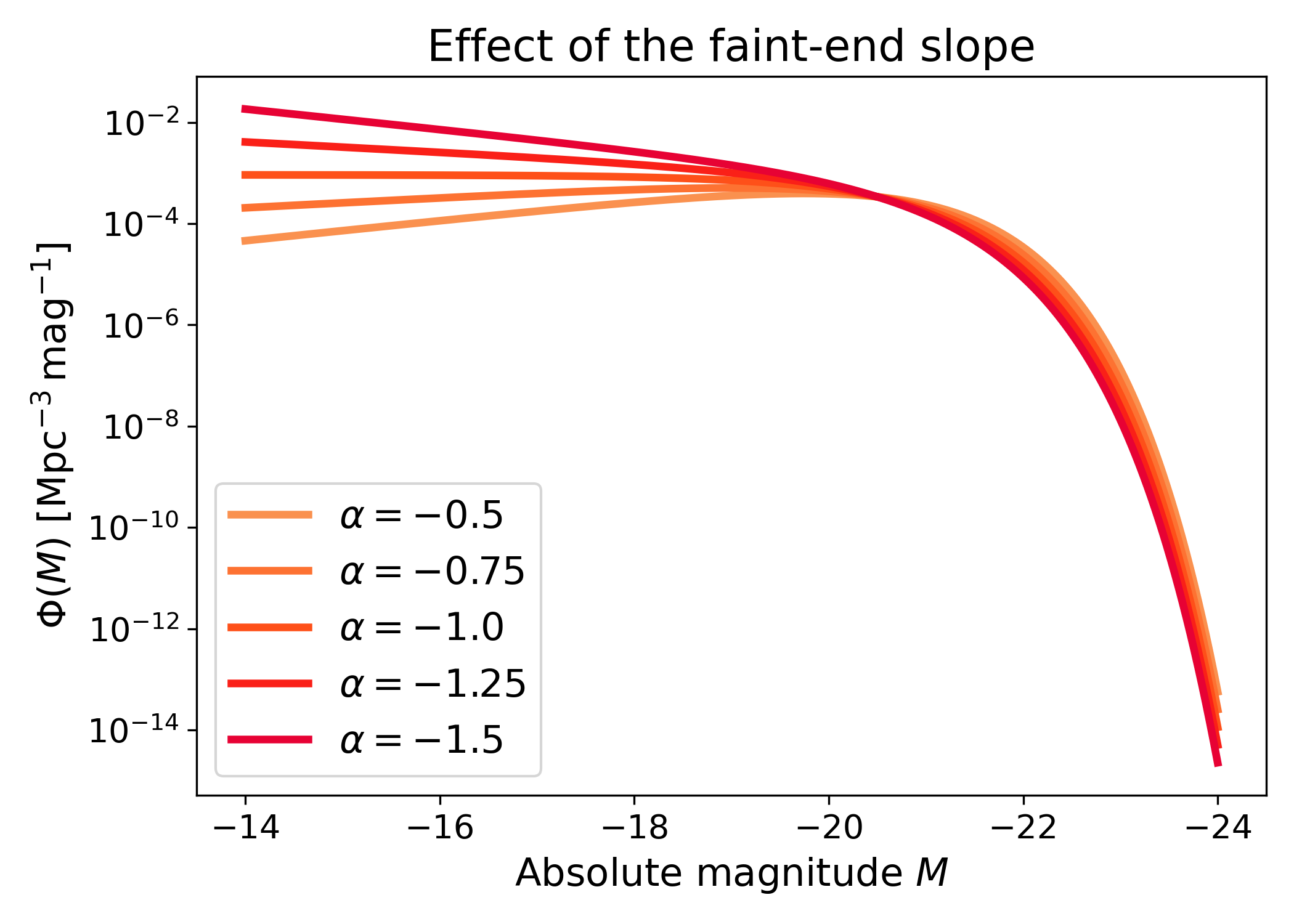
Comparing Schechter slopes#
Changing \(\alpha\) modifies the faint-end behaviour of the luminosity function. More negative values of \(\alpha\) produce a steeper rise toward faint magnitudes, while less negative values give a shallower faint-end population.
This comparison keeps the other Schechter parameters fixed so that the effect of \(\alpha\) is isolated. This is useful because the faint-end slope often controls how strongly low-luminosity galaxies contribute to integrated quantities such as number density or luminosity density.
import numpy as np
import matplotlib.pyplot as plt
import cmasher as cmr

from lfkit import LuminosityFunction

LABEL_SIZE = 15
TICK_SIZE = 13
TITLE_SIZE = 17
LEGEND_SIZE = 15

absolute_mag = np.linspace(-24.0, -14.0, 500)
alphas = [-0.5, -0.75, -1.0, -1.25, -1.5]

colors = cmr.take_cmap_colors(
        "cmr.guppy",
        len(alphas),
        cmap_range=(0.0, 0.2)
    )

fig, ax = plt.subplots(figsize=(7.0, 5.0))

for alpha, color in zip(alphas, colors):
    lf = LuminosityFunction.schechter(
        phi_star=1.0e-3,
        m_star=-20.5,
        alpha=alpha,
    )
    ax.plot(
        absolute_mag,
        lf.phi(absolute_mag),
        lw=3,
        color=color,
        label=rf"$\alpha={alpha}$",
    )

ax.set_yscale("log")
ax.invert_xaxis()
ax.set_xlabel("Absolute magnitude $M$", fontsize=LABEL_SIZE)
ax.set_ylabel(
    r"$\Phi(M)$ [$\mathrm{Mpc}^{-3}\,\mathrm{mag}^{-1}$]",
    fontsize=LABEL_SIZE,
)
ax.set_title("Effect of the faint-end slope", fontsize=TITLE_SIZE)
ax.tick_params(axis="both", labelsize=TICK_SIZE)
ax.legend(frameon=True, fontsize=LEGEND_SIZE, loc="best")
plt.tight_layout()
(png)

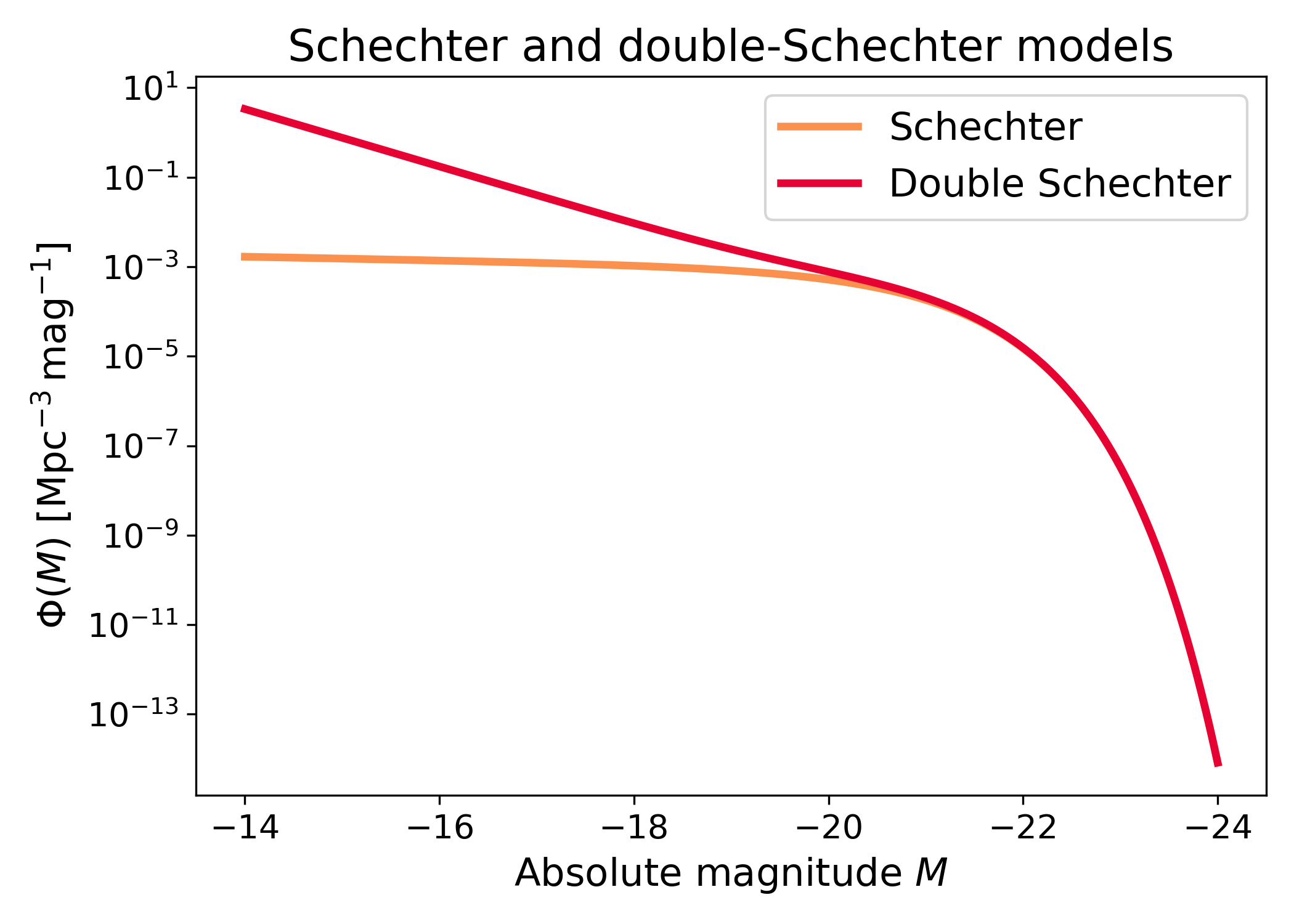
Double Schechter luminosity function#
The API also exposes a double-Schechter constructor. This is useful for models that need extra flexibility at the faint end while retaining a Schechter-like bright-end cutoff.
The double-Schechter form adds a second faint-end component. This can represent a luminosity function whose faint population cannot be captured well by one single Schechter slope.
import numpy as np
import matplotlib.pyplot as plt
import cmasher as cmr

from lfkit import LuminosityFunction

LABEL_SIZE = 15
TICK_SIZE = 13
TITLE_SIZE = 17
LEGEND_SIZE = 15

single = LuminosityFunction.schechter(
    phi_star=1.0e-3,
    m_star=-20.5,
    alpha=-1.1,
)

double = LuminosityFunction.double_schechter(
    phi_star=1.0e-3,
    m_star=-20.5,
    alpha=-1.1,
    beta=-1.5,
    m_transition=-19.5,
)

absolute_mag = np.linspace(-24.0, -14.0, 500)
colors = cmr.take_cmap_colors("cmr.guppy", 2, cmap_range=(0.0, 0.2))

fig, ax = plt.subplots(figsize=(7.0, 5.0))
ax.plot(
    absolute_mag,
    single.phi(absolute_mag),
    lw=3,
    color=colors[0],
    label="Schechter",
)
ax.plot(
    absolute_mag,
    double.phi(absolute_mag),
    lw=3,
    color=colors[1],
    label="Double Schechter",
)

ax.set_yscale("log")
ax.invert_xaxis()
ax.set_xlabel("Absolute magnitude $M$", fontsize=LABEL_SIZE)
ax.set_ylabel(
    r"$\Phi(M)$ [$\mathrm{Mpc}^{-3}\,\mathrm{mag}^{-1}$]",
    fontsize=LABEL_SIZE,
)
ax.set_title("Schechter and double-Schechter models", fontsize=TITLE_SIZE)
ax.tick_params(axis="both", labelsize=TICK_SIZE)
ax.legend(frameon=True, fontsize=LEGEND_SIZE, loc="best")
plt.tight_layout()
(png)

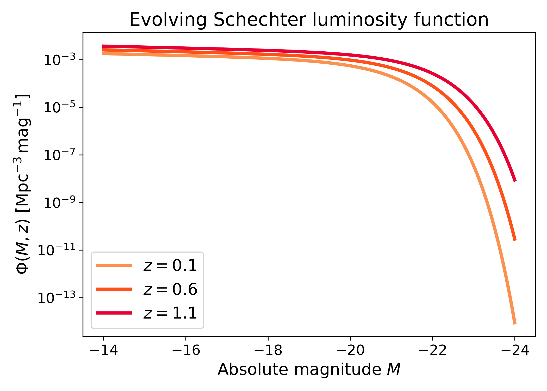
Evolving Schechter luminosity function#
An evolving Schechter luminosity function lets the Schechter parameters depend on redshift through LFKit’s registered parameter models. This is useful when the same LF object should evaluate \(\Phi(M, z)\) at many redshifts.
The curves below show how the predicted luminosity function changes when the normalization, characteristic magnitude, or slope evolve with redshift. This is the model form used when the galaxy population is not assumed to be fixed across cosmic time.
import numpy as np
import matplotlib.pyplot as plt
import cmasher as cmr

from lfkit import LuminosityFunction

LABEL_SIZE = 15
TICK_SIZE = 13
TITLE_SIZE = 17
LEGEND_SIZE = 15

lf = LuminosityFunction.evolving_schechter(
    phi_model="linear_p",
    phi_kwargs={"phi_0_star": 1.0e-3, "p": 0.7},
    m_star_model="linear_q",
    m_star_kwargs={"m_0_star": -20.5, "q": 0.8, "z_ref": 0.1},
    alpha_model="constant",
    alpha_kwargs={"alpha": -1.1},
)

absolute_mag = np.linspace(-24.0, -14.0, 500)
redshifts = [0.1, 0.6, 1.1]
colors = cmr.take_cmap_colors(
        "cmr.guppy",
        len(redshifts),
        cmap_range=(0.0, 0.2)
    )

fig, ax = plt.subplots(figsize=(7.0, 5.0))

for z_value, color in zip(redshifts, colors):
    phi = lf.phi(absolute_mag, z_value)
    ax.plot(
        absolute_mag,
        phi,
        lw=3,
        color=color,
        label=rf"$z={z_value}$",
    )

ax.set_yscale("log")
ax.invert_xaxis()
ax.set_xlabel("Absolute magnitude $M$", fontsize=LABEL_SIZE)
ax.set_ylabel(
    r"$\Phi(M, z)$ [$\mathrm{Mpc}^{-3}\,\mathrm{mag}^{-1}$]",
    fontsize=LABEL_SIZE,
)
ax.set_title("Evolving Schechter luminosity function", fontsize=TITLE_SIZE)
ax.tick_params(axis="both", labelsize=TICK_SIZE)
ax.legend(frameon=True, fontsize=LEGEND_SIZE, loc="best")
plt.tight_layout()
(png)
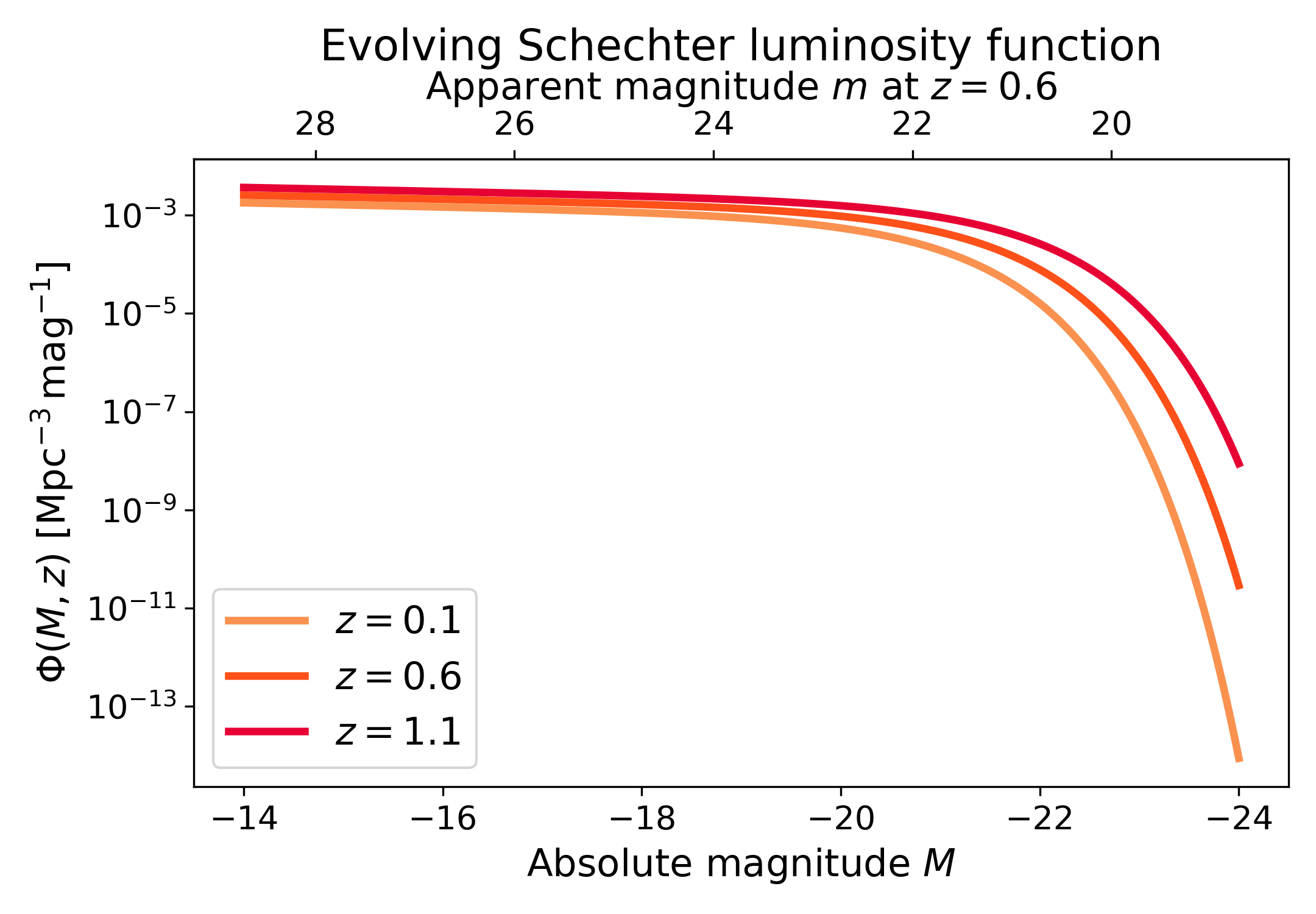
Evolving Schechter luminosity function with apparent magnitude axis#
The evolving Schechter model is evaluated as \(\Phi(M, z)\). A secondary x-axis can show the apparent magnitude corresponding to the absolute magnitude range at a chosen reference luminosity distance.
Here, the curves are evaluated at several redshifts, while the upper apparent magnitude axis is defined for the reference redshift \(z=0.6\). This keeps the bottom axis model-native and avoids mixing several different distance-redshift mappings into one top axis. The top axis should therefore be read as a reference guide, not as a separate conversion for every curve.
import numpy as np
import matplotlib.pyplot as plt
import cmasher as cmr

from lfkit import LuminosityFunction

LABEL_SIZE = 15
TICK_SIZE = 13
TITLE_SIZE = 17
LEGEND_SIZE = 15

lf = LuminosityFunction.evolving_schechter(
    phi_model="linear_p",
    phi_kwargs={"phi_0_star": 1.0e-3, "p": 0.7},
    m_star_model="linear_q",
    m_star_kwargs={"m_0_star": -20.5, "q": 0.8, "z_ref": 0.1},
    alpha_model="constant",
    alpha_kwargs={"alpha": -1.1},
)

absolute_mag = np.linspace(-24.0, -14.0, 500)
redshifts = [0.1, 0.6, 1.1]

reference_redshift = 0.6
luminosity_distance_mpc = {
    0.1: 460.0,
    0.6: 3500.0,
    1.1: 7600.0,
}
reference_luminosity_distance_mpc = luminosity_distance_mpc[reference_redshift]

colors = cmr.take_cmap_colors(
        "cmr.guppy",
        len(redshifts),
        cmap_range=(0.0, 0.2)
    )

fig, ax = plt.subplots(figsize=(7.2, 5.0))

for z_value, color in zip(redshifts, colors):
    phi = lf.phi(absolute_mag, z_value)
    ax.plot(
        absolute_mag,
        phi,
        lw=3,
        color=color,
        label=rf"$z={z_value}$",
    )

secax = ax.secondary_xaxis(
    "top",
    functions=(
        lambda absolute_mag: lf.magnitudes.apparent_from_luminosity_distance(
            absolute_mag,
            reference_luminosity_distance_mpc,
        ),
        lambda apparent_mag: lf.magnitudes.absolute_from_luminosity_distance(
            apparent_mag,
            reference_luminosity_distance_mpc,
        ),
    ),
)

ax.set_yscale("log")
ax.invert_xaxis()
ax.set_xlabel("Absolute magnitude $M$", fontsize=LABEL_SIZE)
ax.set_ylabel(
    r"$\Phi(M, z)$ [$\mathrm{Mpc}^{-3}\,\mathrm{mag}^{-1}$]",
    fontsize=LABEL_SIZE,
)
ax.set_title(
    "Evolving Schechter luminosity function",
    fontsize=TITLE_SIZE,
    pad=0.5,
)
ax.tick_params(axis="both", labelsize=TICK_SIZE)
ax.legend(frameon=True, fontsize=LEGEND_SIZE, loc="best")

secax.set_xlabel(
    rf"Apparent magnitude $m$ at $z={reference_redshift}$",
    fontsize=LABEL_SIZE,
)
secax.tick_params(axis="x", labelsize=TICK_SIZE)

plt.tight_layout()
(png)
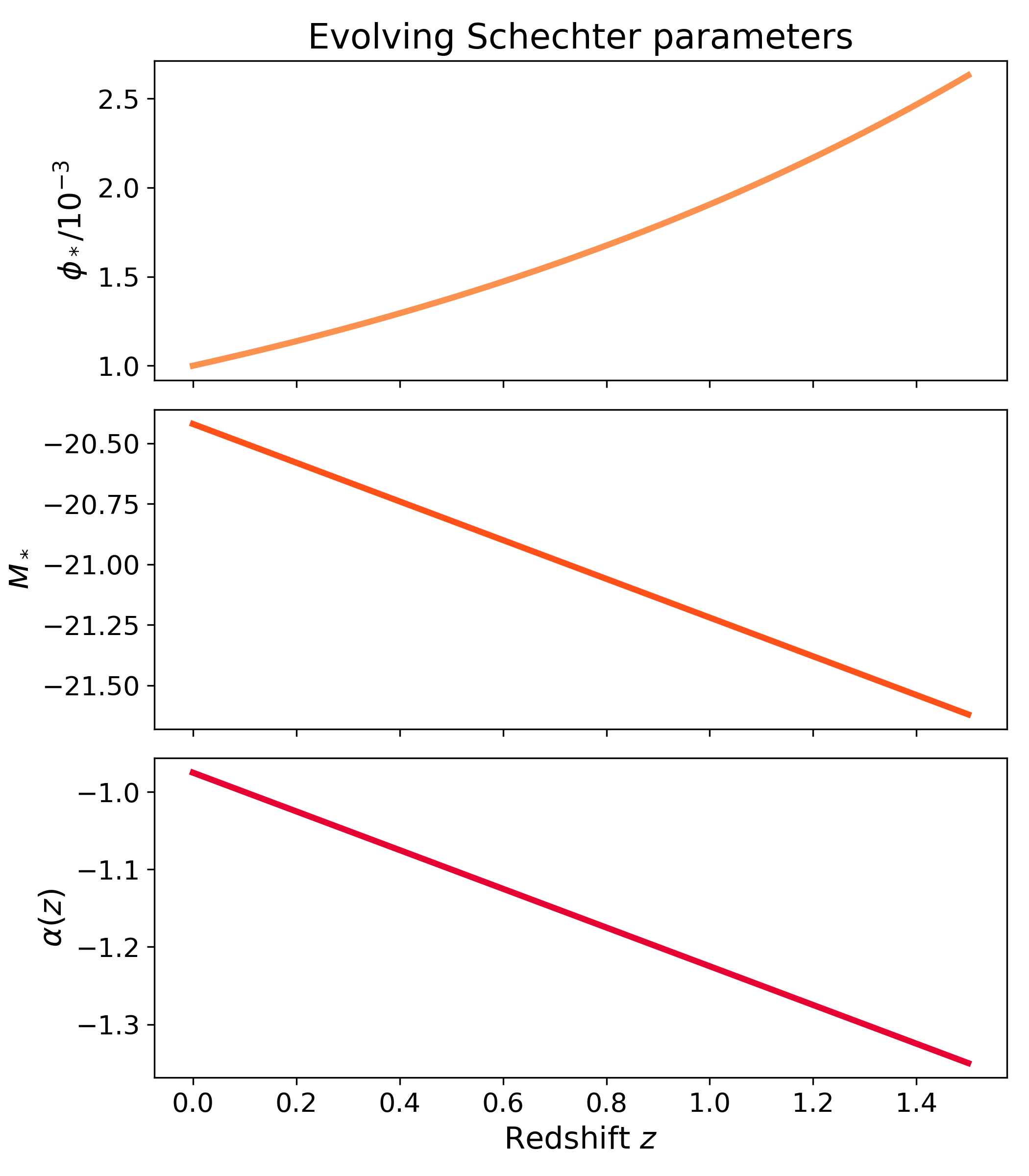
Inspecting evolving parameters#
For evolving models, lfkit.LuminosityFunction.parameters() evaluates the
registered parameter models at the requested redshift. This is useful for
checking the model behaviour before using the LF in number-density or selection
calculations.
Here all three Schechter parameters evolve with redshift, including the faint-end slope \(\alpha(z)\). This diagnostic separates the ingredients of the luminosity function: \(\phi_*\) controls the normalization, \(M_*\) sets the characteristic magnitude, and \(\alpha\) controls the faint-end slope.
import numpy as np
import matplotlib.pyplot as plt
import cmasher as cmr

from lfkit import LuminosityFunction

LABEL_SIZE = 15
TICK_SIZE = 13
TITLE_SIZE = 17

lf = LuminosityFunction.evolving_schechter(
    phi_model="linear_p",
    phi_kwargs={"phi_0_star": 1.0e-3, "p": 0.7},
    m_star_model="linear_q",
    m_star_kwargs={"m_0_star": -20.5, "q": 0.8, "z_ref": 0.1},
    alpha_model="linear",
    alpha_kwargs={"alpha_0": -1.0, "alpha_1": -0.25, "z_ref": 0.1},
)

redshift = np.linspace(0.0, 1.5, 200)
phi_star, m_star, alpha = lf.parameters(redshift)
colors = cmr.take_cmap_colors("cmr.guppy", 3, cmap_range=(0.0, 0.2))

fig, axes = plt.subplots(
    nrows=3,
    ncols=1,
    figsize=(7.0, 8.0),
    sharex=True,
)

axes[0].plot(
    redshift,
    phi_star / 1.0e-3,
    lw=3,
    color=colors[0],
)
axes[0].set_ylabel(r"$\phi_*/10^{-3}$", fontsize=LABEL_SIZE)

axes[1].plot(
    redshift,
    m_star,
    lw=3,
    color=colors[1],
)
axes[1].set_ylabel(r"$M_*$", fontsize=LABEL_SIZE)

axes[2].plot(
    redshift,
    alpha,
    lw=3,
    color=colors[2],
)
axes[2].set_ylabel(r"$\alpha(z)$", fontsize=LABEL_SIZE)
axes[2].set_xlabel("Redshift $z$", fontsize=LABEL_SIZE)

axes[0].set_title("Evolving Schechter parameters", fontsize=TITLE_SIZE)

for axis in axes:
    axis.tick_params(axis="both", labelsize=TICK_SIZE)

plt.tight_layout()
(png)
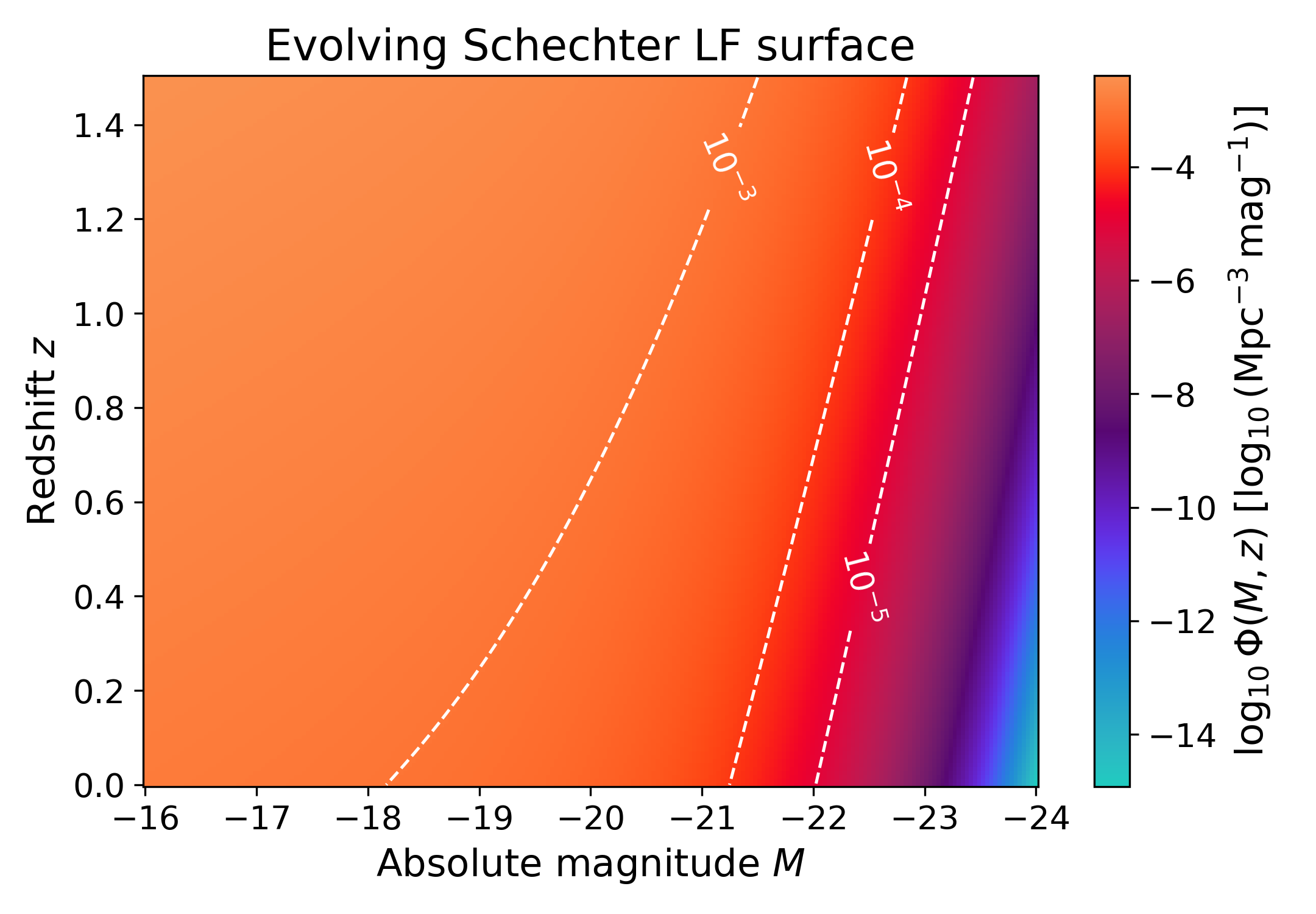
Evolving Schechter surface#
The same evolving model can be shown over the full magnitude-redshift plane. The filled colour scale shows \(\log_{10}\Phi(M, z)\), while contours mark constant abundance levels.
This view is useful for seeing the joint magnitude and redshift dependence in one panel. Horizontal changes show how the luminosity function varies with magnitude, while vertical changes show how the evolving parameters modify the model with redshift.
import numpy as np
import matplotlib.pyplot as plt
import cmasher as cmr

from lfkit import LuminosityFunction

LABEL_SIZE = 15
TICK_SIZE = 13
TITLE_SIZE = 17

lf = LuminosityFunction.evolving_schechter(
    phi_model="linear_p",
    phi_kwargs={"phi_0_star": 1.0e-3, "p": 0.7},
    m_star_model="linear_q",
    m_star_kwargs={"m_0_star": -20.5, "q": 0.8, "z_ref": 0.1},
    alpha_model="constant",
    alpha_kwargs={"alpha": -1.1},
)

absolute_mag = np.linspace(-24.0, -16.0, 220)
redshift = np.linspace(0.0, 1.5, 180)
mag_grid, z_grid = np.meshgrid(absolute_mag, redshift)

phi = lf.phi(mag_grid, z_grid)
log_phi = np.log10(phi)

fig, ax = plt.subplots(figsize=(7.2, 5.0))

mesh = ax.pcolormesh(
    absolute_mag,
    redshift,
    log_phi,
    shading="auto",
    cmap=cmr.get_sub_cmap('cmr.guppy_r', 0.0, 1)
)

contour_levels = [-5.0, -4.0, -3.0, -2.0]
contours = ax.contour(
    absolute_mag,
    redshift,
    log_phi,
    levels=contour_levels,
    colors="white",
    linewidths=1.2,
)
ax.clabel(contours, inline=True, fontsize=TICK_SIZE, fmt=r"$10^{%.0f}$")

ax.invert_xaxis()
ax.set_xlabel("Absolute magnitude $M$", fontsize=LABEL_SIZE)
ax.set_ylabel("Redshift $z$", fontsize=LABEL_SIZE)
ax.set_title("Evolving Schechter LF surface", fontsize=TITLE_SIZE)
ax.tick_params(axis="both", labelsize=TICK_SIZE)

cbar = fig.colorbar(mesh, ax=ax)
cbar.set_label(
    r"$\log_{10}\Phi(M, z)$ "
    r"[$\log_{10}(\mathrm{Mpc}^{-3}\,\mathrm{mag}^{-1})$]",
    fontsize=LABEL_SIZE,
)
cbar.ax.tick_params(labelsize=TICK_SIZE)

plt.tight_layout()
(png)

Other luminosity function parametrizations#
Additional luminosity function parametrizations can be added here as they are implemented in the public API.
Examples may include Saunders or modified-Schechter models, double-power-law forms, lognormal-inspired parametrizations, or other survey-specific luminosity function models. This section is intentionally kept as a placeholder so the page can grow beyond the Schechter family without mixing all models under one flat heading structure.
Available models#
The API can report the registered luminosity function models and parameter models. This is useful for examples, validation, and interactive exploration.
from lfkit import LuminosityFunction

LuminosityFunction.available_models()
LuminosityFunction.available_from_m_models()
LuminosityFunction.available_parameter_models()