 Magnitude integrals#
This page shows how to integrate a bound
lfkit.LuminosityFunction over absolute magnitude.
The examples use the lf.integrals namespace. These methods insert the
luminosity function callable internally, so users only provide the redshift
values, magnitude limits, and any optional weighting functions.
Magnitude integrals are useful when a luminosity function is used to predict number densities, luminosity-weighted summaries, or selected fractions over a finite magnitude range.
The number-density units follow the normalization supplied to the luminosity
function. For example, if phi_star is supplied in
\({\rm Mpc}^{-3}\,{\rm mag}^{-1}\), then magnitude-integrated number
densities have units of \({\rm Mpc}^{-3}\).
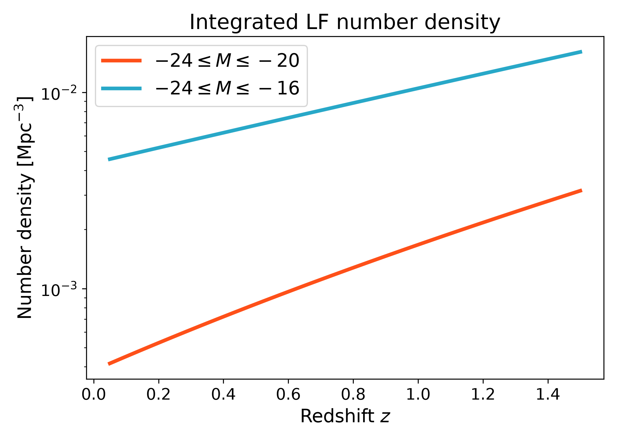
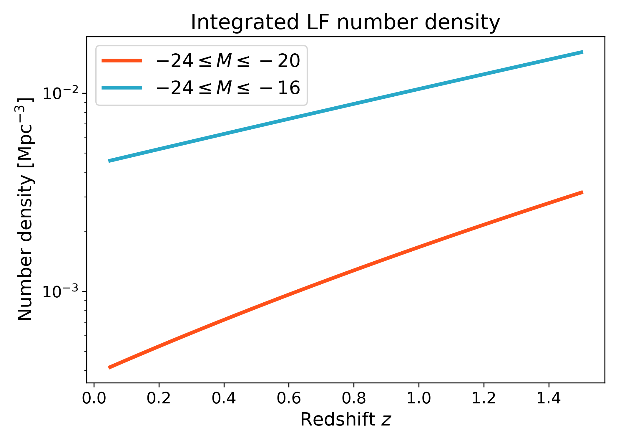
Integrated number density#
The integrated number density is the luminosity function integrated over a finite absolute magnitude range. It gives the abundance of galaxies retained by a chosen magnitude selection.
This example compares a bright sample to a broader sample that also includes fainter galaxies. The broader magnitude range gives a larger number density because more of the faint end of the luminosity function is included. In practice, these magnitude limits can be changed to match a survey cut, a science sample definition, or a test range used for model comparisons.
import numpy as np
import matplotlib.pyplot as plt
import cmasher as cmr
from matplotlib.ticker import LogLocator, LogFormatterMathtext

from lfkit import LuminosityFunction

LABEL_SIZE = 15
TICK_SIZE = 13
TITLE_SIZE = 17
LEGEND_SIZE = 15

lf = LuminosityFunction.evolving_schechter(
    phi_model="linear_p",
    phi_kwargs={"phi_0_star": 1.0e-3, "p": 0.7},
    m_star_model="linear_q",
    m_star_kwargs={"m_0_star": -20.5, "q": 0.8, "z_ref": 0.1},
    alpha_model="constant",
    alpha_kwargs={"alpha": -1.1},
)

redshift = np.linspace(0.05, 1.5, 180)

n_bright = lf.integrals.number_density(
    redshift,
    m_bright=-24.0,
    m_faint=-20.0,
    n_m=800,
)

n_total = lf.integrals.number_density(
    redshift,
    m_bright=-24.0,
    m_faint=-16.0,
    n_m=800,
)

red = cmr.take_cmap_colors("cmr.guppy", 3, cmap_range=(0.0, 0.2))[1]
blue = cmr.take_cmap_colors("cmr.guppy", 3, cmap_range=(0.8, 1.0))[1]

fig, ax = plt.subplots(figsize=(7.0, 5.0))
ax.plot(
    redshift,
    n_bright,
    lw=3,
    color=red,
    label=r"$-24 \leq M \leq -20$",
)
ax.plot(
    redshift,
    n_total,
    lw=3,
    color=blue,
    label=r"$-24 \leq M \leq -16$",
)

ax.set_yscale("log")
ax.yaxis.set_major_locator(LogLocator(base=10.0, numticks=5))
ax.yaxis.set_major_formatter(LogFormatterMathtext(base=10.0))
ax.yaxis.set_minor_locator(
    LogLocator(base=10.0, subs=np.arange(2, 10) * 0.1, numticks=12)
)

ax.set_xlabel("Redshift $z$", fontsize=LABEL_SIZE)
ax.set_ylabel(r"Number density [$\mathrm{Mpc}^{-3}$]", fontsize=LABEL_SIZE)
ax.set_title("Integrated LF number density", fontsize=TITLE_SIZE)
ax.tick_params(axis="both", labelsize=TICK_SIZE)
ax.legend(frameon=True, fontsize=LEGEND_SIZE, loc="best")
plt.tight_layout()
(png)
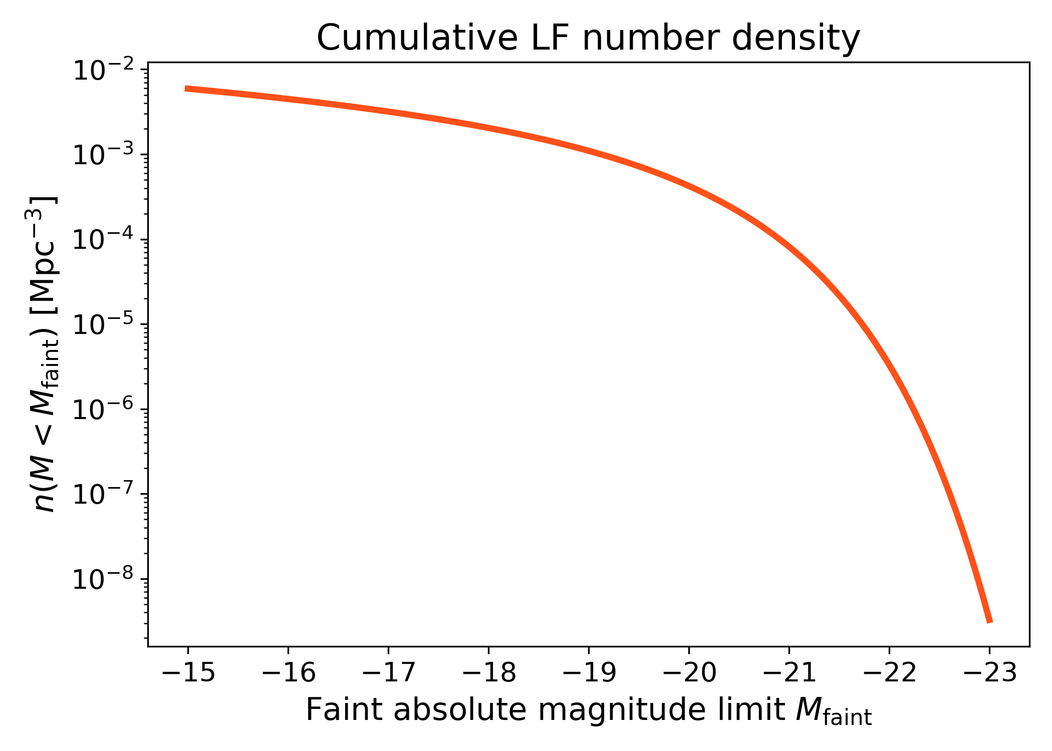
Cumulative number density#
The number density can also be viewed as a cumulative function of the faint absolute magnitude limit. Here the bright limit is held fixed, while the faint limit is moved across the luminosity function.
This diagnostic is useful for checking how much faint galaxies contribute to the total abundance. As the faint limit moves to less negative magnitudes, more galaxies are included and the cumulative number density increases. The shape of this curve shows where most of the abundance is coming from in magnitude space.
import numpy as np
import matplotlib.pyplot as plt
import cmasher as cmr

from lfkit import LuminosityFunction

LABEL_SIZE = 15
TICK_SIZE = 13
TITLE_SIZE = 17

lf = LuminosityFunction.schechter(
    phi_star=1.0e-3,
    m_star=-20.5,
    alpha=-1.1,
)

magnitude_limits = np.linspace(-23.0, -15.0, 120)

number_density = lf.integrals.number_density(
    0.0,
    m_bright=-25.0,
    m_faint=magnitude_limits,
    n_m=800,
)

fig, ax = plt.subplots(figsize=(7.0, 5.0))
ax.plot(
    magnitude_limits,
    number_density,
    lw=3,
    color=cmr.take_cmap_colors("cmr.guppy", 3, cmap_range=(0.0, 0.2))[1],
)

ax.set_yscale("log")
ax.invert_xaxis()
ax.set_xlabel(
    r"Faint absolute magnitude limit $M_{\rm faint}$",
    fontsize=LABEL_SIZE,
)
ax.set_ylabel(
    r"$n(M < M_{\rm faint})$ [$\mathrm{Mpc}^{-3}$]",
    fontsize=LABEL_SIZE,
)
ax.set_title("Cumulative LF number density", fontsize=TITLE_SIZE)
ax.tick_params(axis="both", labelsize=TICK_SIZE)
plt.tight_layout()
(png)
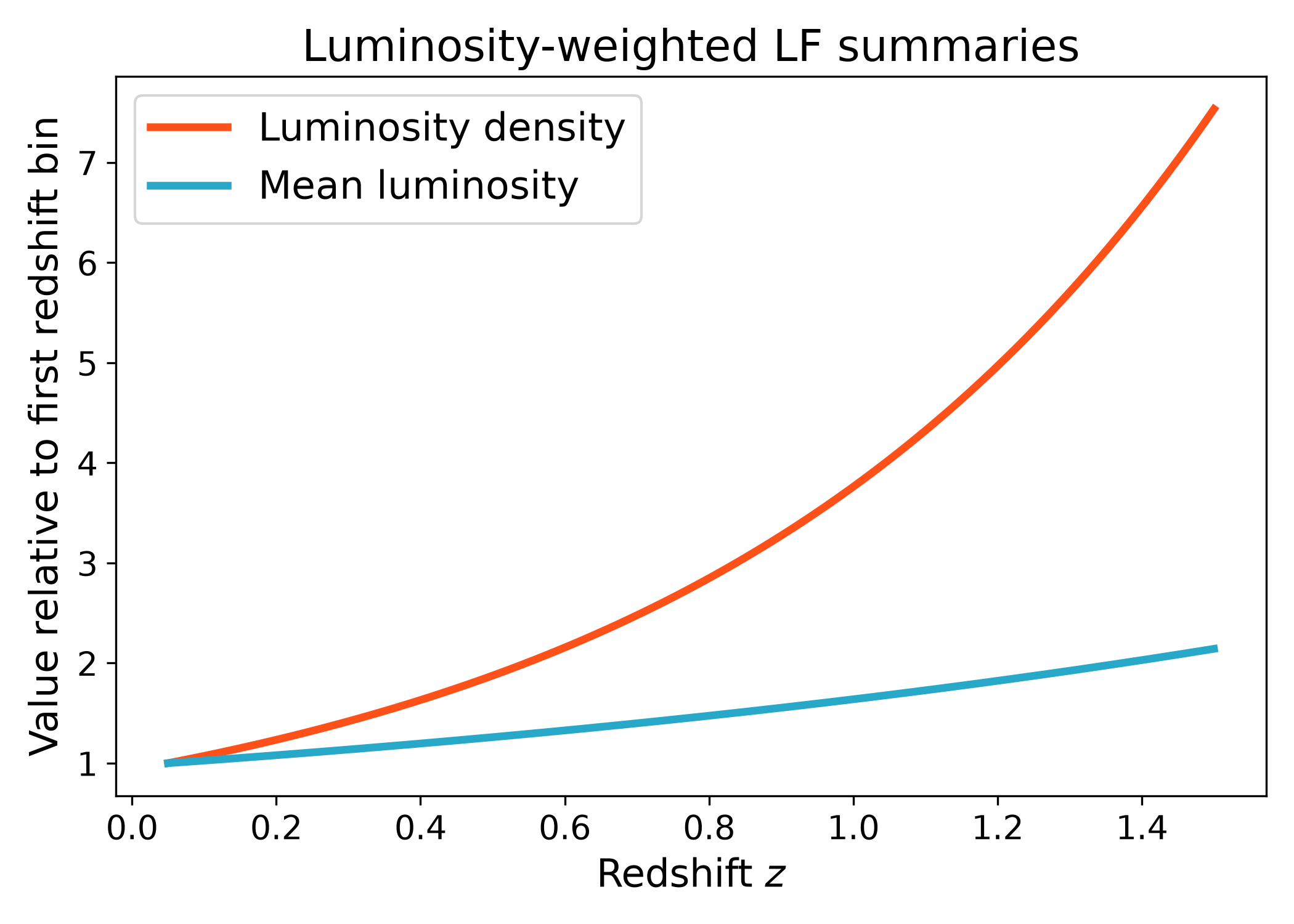
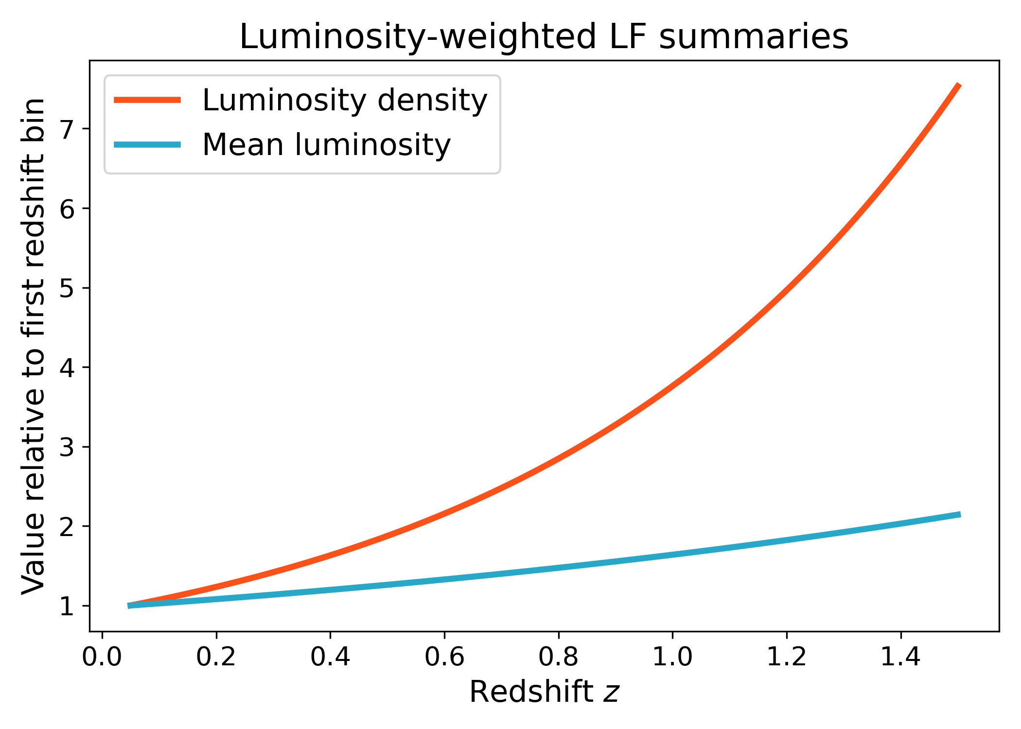
Luminosity density and mean luminosity#
The same namespace can compute luminosity-weighted summaries such as luminosity density and mean luminosity over a selected magnitude range. These quantities weight the luminosity function by luminosity before integrating, so they are more sensitive to the bright end than the number density alone.
The curves below are normalized by their first redshift value to emphasize the relative redshift trend rather than the absolute normalization. This makes it easier to compare how the luminosity density and mean luminosity evolve across redshift for the same underlying luminosity function model.
import numpy as np
import matplotlib.pyplot as plt
import cmasher as cmr

from lfkit import LuminosityFunction

LABEL_SIZE = 15
TICK_SIZE = 13
TITLE_SIZE = 17
LEGEND_SIZE = 15

lf = LuminosityFunction.evolving_schechter(
    phi_model="linear_p",
    phi_kwargs={"phi_0_star": 1.0e-3, "p": 0.7},
    m_star_model="linear_q",
    m_star_kwargs={"m_0_star": -20.5, "q": 0.8, "z_ref": 0.1},
    alpha_model="constant",
    alpha_kwargs={"alpha": -1.1},
)

redshift = np.linspace(0.05, 1.5, 180)

luminosity_density = lf.integrals.luminosity_density(
    redshift,
    m_bright=-24.0,
    m_faint=-16.0,
    n_m=800,
)

mean_luminosity = lf.integrals.mean_luminosity(
    redshift,
    m_bright=-24.0,
    m_faint=-16.0,
    n_m=800,
)

red = cmr.take_cmap_colors("cmr.guppy", 3, cmap_range=(0.0, 0.2))[1]
blue = cmr.take_cmap_colors("cmr.guppy", 3, cmap_range=(0.8, 1.0))[1]

fig, ax = plt.subplots(figsize=(7.0, 5.0))
ax.plot(
    redshift,
    luminosity_density / luminosity_density[0],
    lw=3,
    color=red,
    label="Luminosity density",
)
ax.plot(
    redshift,
    mean_luminosity / mean_luminosity[0],
    lw=3,
    color=blue,
    label="Mean luminosity",
)

ax.set_xlabel("Redshift $z$", fontsize=LABEL_SIZE)
ax.set_ylabel("Value relative to first redshift bin", fontsize=LABEL_SIZE)
ax.set_title("Luminosity-weighted LF summaries", fontsize=TITLE_SIZE)
ax.tick_params(axis="both", labelsize=TICK_SIZE)
ax.legend(frameon=True, fontsize=LEGEND_SIZE, loc="best")
plt.tight_layout()
(png)
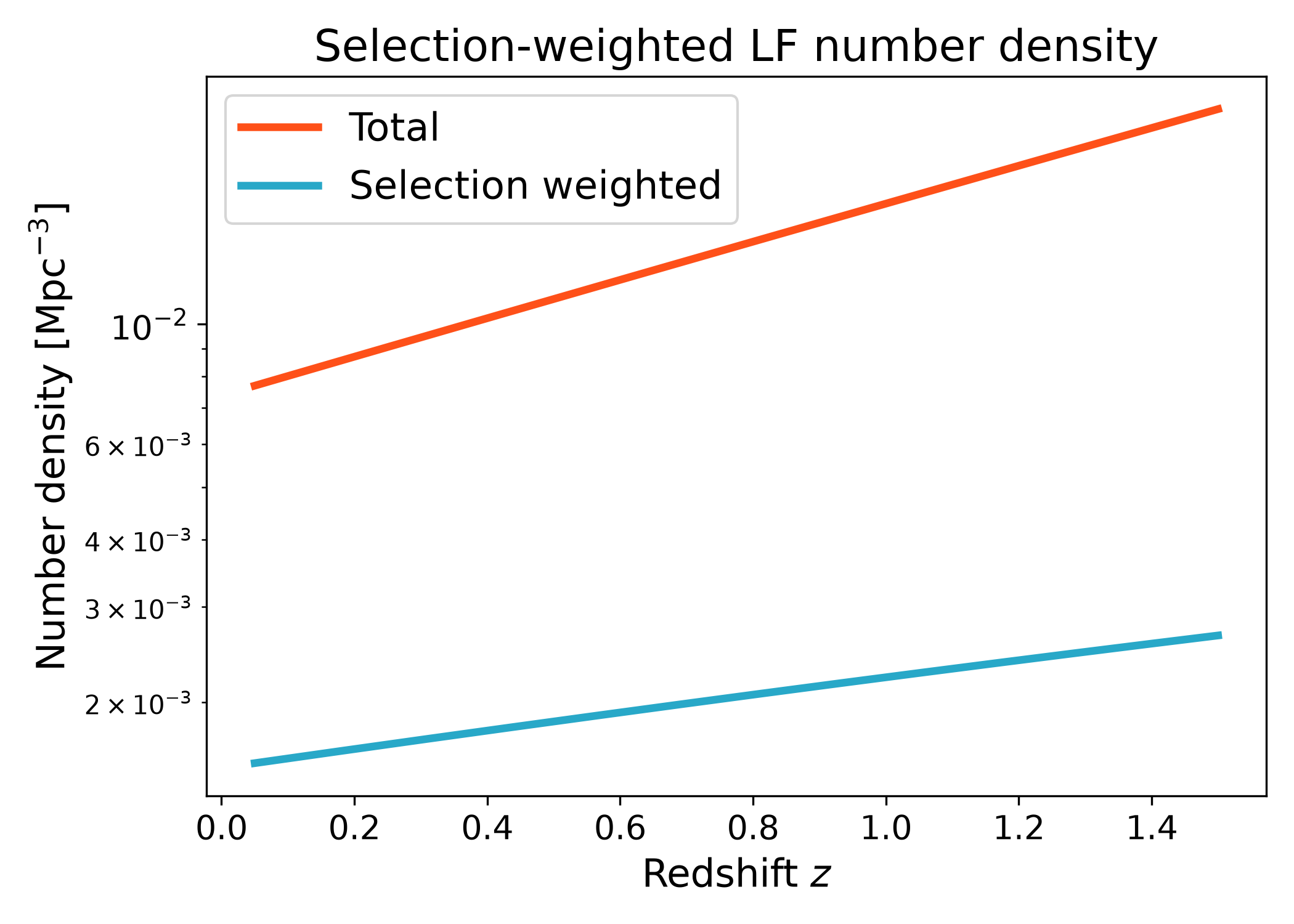
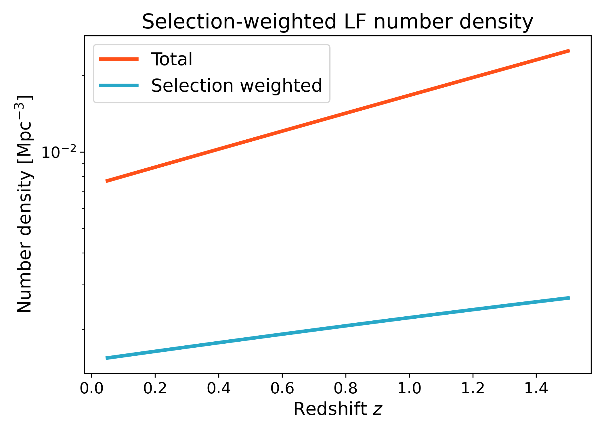
Selection-weighted number density#
Selection weights can be applied directly through the integrals API. This is useful when a sample is not selected by a hard magnitude cut alone, but instead has a gradual completeness, targeting, or selection probability.
This example uses a smooth user-defined selection function in absolute magnitude. The function used here is only one possible choice: users can replace it with any callable that returns a selection weight for absolute magnitude and redshift. The selected number density is lower than the total number density because the selection downweights part of the magnitude range instead of retaining every galaxy equally.
import numpy as np
import matplotlib.pyplot as plt
import cmasher as cmr
from matplotlib.ticker import LogLocator, LogFormatterMathtext

from lfkit import LuminosityFunction

LABEL_SIZE = 15
TICK_SIZE = 13
TITLE_SIZE = 17
LEGEND_SIZE = 15

lf = LuminosityFunction.evolving_schechter(
    phi_model="linear_p",
    phi_kwargs={"phi_0_star": 1.0e-3, "p": 0.7},
    m_star_model="linear_q",
    m_star_kwargs={"m_0_star": -20.5, "q": 0.8, "z_ref": 0.1},
    alpha_model="constant",
    alpha_kwargs={"alpha": -1.1},
)

redshift = np.linspace(0.05, 1.5, 180)

def soft_selection(absolute_mag, z):
    limiting_mag = -18.5 - 1.2 * z
    width = 0.35
    return 1.0 / (1.0 + np.exp((absolute_mag - limiting_mag) / width))

n_total = lf.integrals.number_density(
    redshift,
    m_bright=-24.0,
    m_faint=-14.0,
    n_m=800,
)

n_selected = lf.integrals.selection_weighted_number_density(
    redshift,
    selection_fn=soft_selection,
    m_bright=-24.0,
    m_faint=-14.0,
    n_m=800,
)

red = cmr.take_cmap_colors("cmr.guppy", 3, cmap_range=(0.0, 0.2))[1]
blue = cmr.take_cmap_colors("cmr.guppy", 3, cmap_range=(0.8, 1.0))[1]

fig, ax = plt.subplots(figsize=(7.0, 5.0))
ax.plot(redshift, n_total, lw=3, color=red, label="Total")
ax.plot(
    redshift,
    n_selected,
    lw=3,
    color=blue,
    label="Selection weighted",
)

ax.set_yscale("log")
ax.yaxis.set_major_locator(LogLocator(base=10.0, numticks=5))
ax.yaxis.set_major_formatter(LogFormatterMathtext(base=10.0))
ax.yaxis.set_minor_locator(
    LogLocator(base=10.0, subs=np.arange(2, 10) * 0.1, numticks=12)
)

ax.set_xlabel("Redshift $z$", fontsize=LABEL_SIZE)
ax.set_ylabel(r"Number density [$\mathrm{Mpc}^{-3}$]", fontsize=LABEL_SIZE)
ax.set_title("Selection-weighted LF number density", fontsize=TITLE_SIZE)
ax.tick_params(axis="both", labelsize=TICK_SIZE)
ax.legend(frameon=True, fontsize=LEGEND_SIZE, loc="best")
plt.tight_layout()
(png)
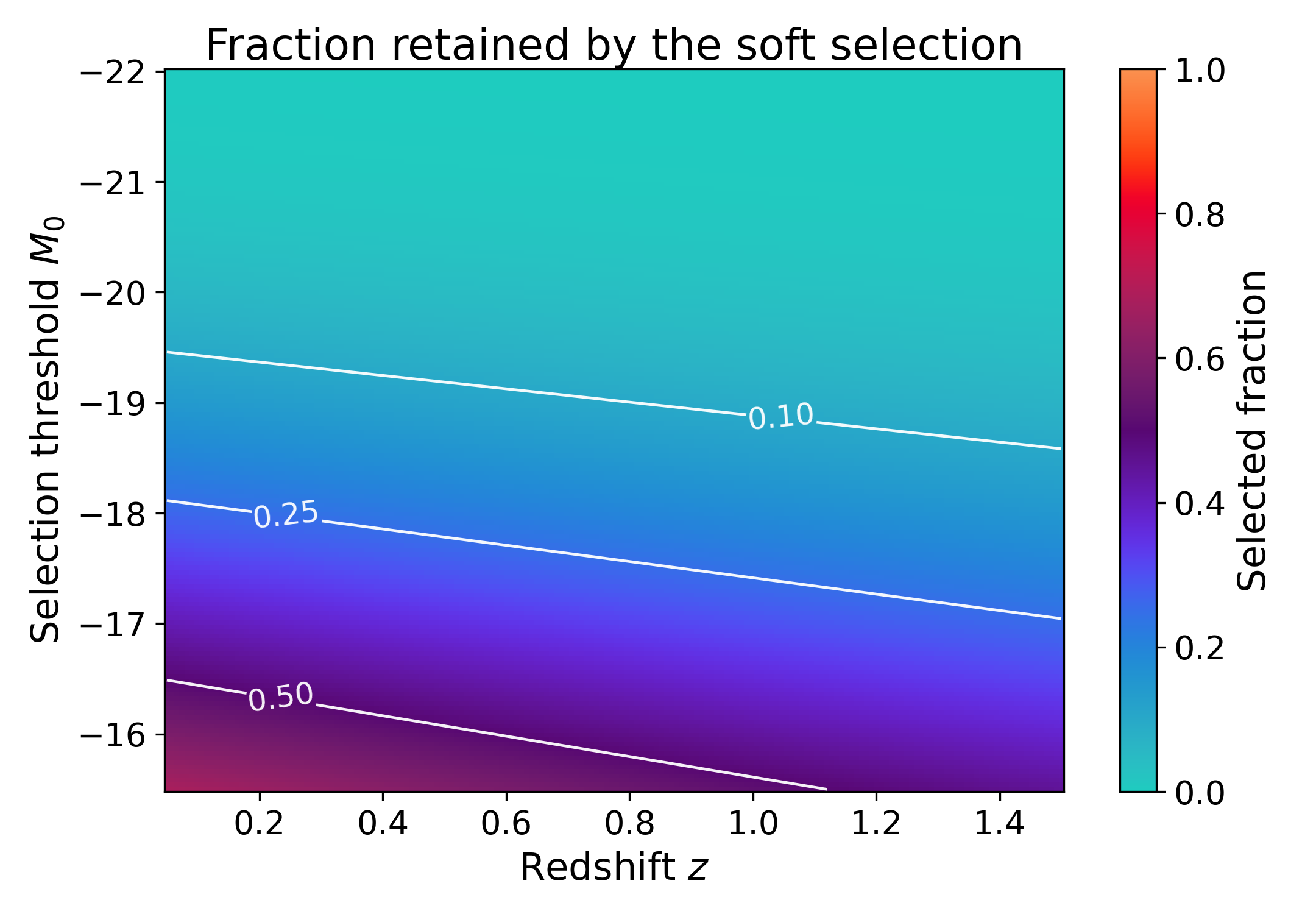
Selection fraction#
The selected fraction is the ratio between the selection-weighted number density and the total number density over the same reference magnitude range. It is a dimensionless diagnostic of how much of the available luminosity function remains after applying a selection function.
This diagnostic is useful for checking how strongly a soft selection changes the effective sample abundance as a function of redshift. A value close to one means that most of the luminosity function within the reference magnitude range is retained, while a value close to zero means that the selection removes most of the available population.
The surface below repeats the calculation for several values of the selection threshold. For each threshold, the code defines a smooth user-controlled selection function and computes the retained fraction relative to the same total number density. Brighter thresholds retain a smaller fraction of the luminosity function, while fainter thresholds retain more of the reference magnitude range. The contours mark constant retained fractions.
In this example the effective limiting magnitude becomes brighter with redshift, so the retained fraction generally decreases toward larger redshift at fixed threshold. Moving to fainter threshold values increases the retained fraction because more of the faint end of the luminosity function passes the selection. Users can replace the threshold model, redshift dependence, or width of the soft transition to represent a different survey selection.
import numpy as np
import matplotlib.pyplot as plt
import cmasher as cmr

from lfkit import LuminosityFunction

LABEL_SIZE = 15
TICK_SIZE = 13
TITLE_SIZE = 17

lf = LuminosityFunction.evolving_schechter(
    phi_model="linear_p",
    phi_kwargs={"phi_0_star": 1.0e-3, "p": 0.7},
    m_star_model="linear_q",
    m_star_kwargs={"m_0_star": -20.5, "q": 0.8, "z_ref": 0.1},
    alpha_model="constant",
    alpha_kwargs={"alpha": -1.1},
)

redshift = np.linspace(0.05, 1.5, 180)
selection_thresholds = np.linspace(-22.0, -15.5, 160)

n_total = lf.integrals.number_density(
    redshift,
    m_bright=-24.0,
    m_faint=-14.0,
    n_m=800,
)

selected_fraction = []

for threshold in selection_thresholds:

    def soft_selection(absolute_mag, z, threshold=threshold):
        limiting_mag = threshold - 1.2 * z
        width = 0.35
        return 1.0 / (1.0 + np.exp((absolute_mag - limiting_mag) / width))

    n_selected = lf.integrals.selection_weighted_number_density(
        redshift,
        selection_fn=soft_selection,
        m_bright=-24.0,
        m_faint=-14.0,
        n_m=800,
    )

    selected_fraction.append(n_selected / n_total)

selected_fraction = np.asarray(selected_fraction)

fig, ax = plt.subplots(figsize=(7.2, 5.0))

mesh = ax.pcolormesh(
    redshift,
    selection_thresholds,
    selected_fraction,
    shading="auto",
    cmap=cmr.get_sub_cmap("cmr.guppy_r", 0.0, 1.0),
    vmin=0.0,
    vmax=1.0,
)

contour_levels = [0.1, 0.25, 0.5, 0.75, 0.9]

contours = ax.contour(
    redshift,
    selection_thresholds,
    selected_fraction,
    levels=contour_levels,
    colors="white",
    linewidths=1.1,
    alpha=0.95,
)

ax.clabel(
    contours,
    inline=True,
    fontsize=TICK_SIZE - 1,
    fmt="%.2f",
)

ax.invert_yaxis()
ax.set_xlabel("Redshift $z$", fontsize=LABEL_SIZE)
ax.set_ylabel(r"Selection threshold $M_0$", fontsize=LABEL_SIZE)
ax.set_title(
    "Fraction retained by the soft selection",
    fontsize=TITLE_SIZE,
    pad=0.5,
)
ax.tick_params(axis="both", labelsize=TICK_SIZE)

cbar = fig.colorbar(mesh, ax=ax)
cbar.set_label("Selected fraction", fontsize=LABEL_SIZE)
cbar.ax.tick_params(labelsize=TICK_SIZE)

plt.tight_layout()
(png)