 Conditional luminosity functions#
This page shows how to evaluate conditional luminosity functions with LFKit’s public API. A conditional luminosity function describes the abundance of galaxies as a function of absolute magnitude while allowing the model to depend on another variable.
A conditional luminosity function has the form \(\Phi(M \mid x)\), where \(M\) is absolute magnitude and \(x\) is the conditioning variable. The quantity
is the number density of galaxies with absolute magnitudes between \(M\) and \(M+dM\) at fixed \(x\). The conditioning variable is generic: it can represent redshift, halo mass, environment, galaxy type, richness, stellar mass, or another quantity.
LFKit exposes conditional luminosity functions through
lfkit.ConditionalLuminosityFunction. Each constructor returns a
luminosity function object that can be evaluated with
lf.phi and integrated through the usual lf.integrals namespace.
The examples below use redshift as the conditioning variable because this is
the most common use case for luminosity function evolution. In that case,
\(\Phi(M \mid z)\) describes how the magnitude distribution of galaxies
changes with redshift. The same API can be used with any other conditioning
variable by replacing z with the desired quantity.
The examples include:
a conditional Schechter luminosity function,
a conditional Schechter model using callable parameter evolution,
a lognormal component,
a two-component lognormal plus modified-Schechter model,
integrated number densities and component fractions,
a halo-mass conditional example,
selection-limited number densities.
The number-density units follow the normalization supplied to the luminosity function. For example, if the amplitudes are supplied in \({\rm Mpc}^{-3}\,{\rm mag}^{-1}\), then \(\Phi(M \mid z)\) has units of \({\rm Mpc}^{-3}\,{\rm mag}^{-1}\).
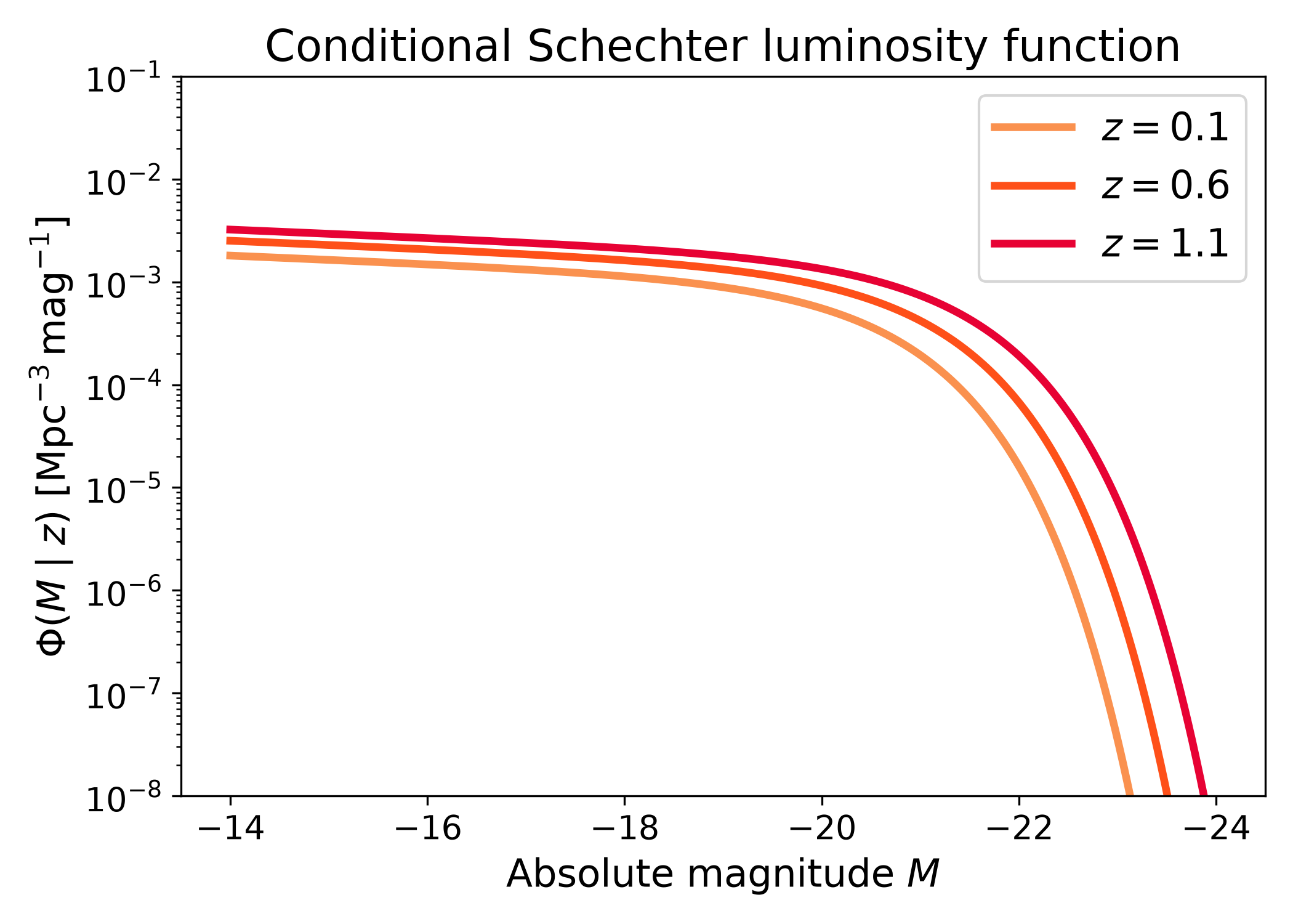
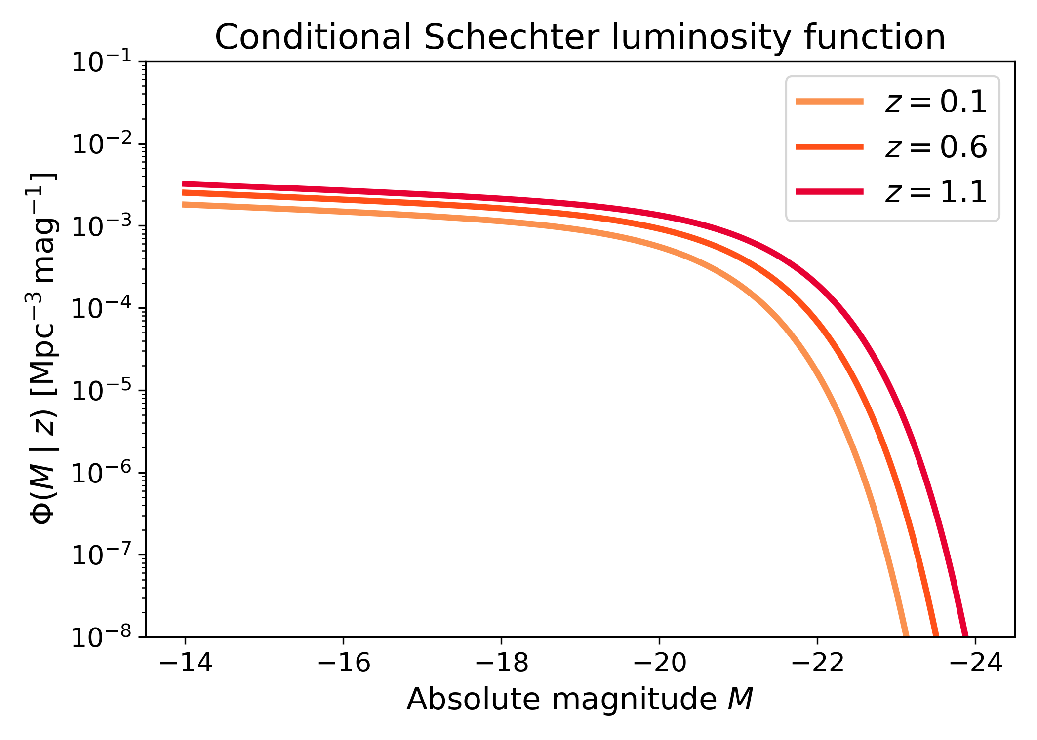
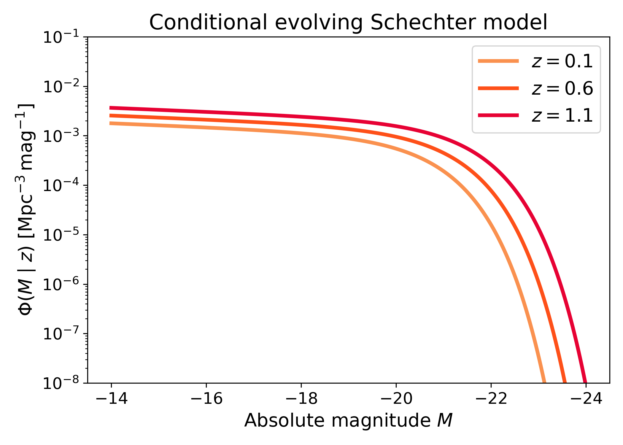
Conditional Schechter luminosity function#
A conditional Schechter luminosity function is a Schechter model whose parameters depend on an external variable. Instead of using one fixed normalization, characteristic magnitude, and faint-end slope, the model can let one or more of these quantities vary with the condition.
This example uses redshift as the condition. The normalization \(\phi_\star(z)\) and characteristic magnitude \(M_\star(z)\) evolve with redshift, while the faint-end slope \(\alpha\) is kept fixed. Each curve is therefore a Schechter luminosity function at one redshift. Comparing the curves shows how the abundance and bright-end turnover shift as the population evolves.
import numpy as np
import matplotlib.pyplot as plt
import cmasher as cmr

from lfkit import ConditionalLuminosityFunction

LABEL_SIZE = 15
TICK_SIZE = 13
TITLE_SIZE = 17
LEGEND_SIZE = 15

absolute_mag = np.linspace(-24.0, -14.0, 500)
redshifts = [0.1, 0.6, 1.1]

colors = cmr.take_cmap_colors(
    "cmr.guppy",
    len(redshifts),
    cmap_range=(0.0, 0.2),
)

lf = ConditionalLuminosityFunction.schechter(
    phi_star=lambda z: 1.0e-3 * (1.0 + z) ** 0.8,
    m_star=lambda z: -20.5 - 0.7 * (z - 0.1),
    alpha=-1.1,
)

fig, ax = plt.subplots(figsize=(7.0, 5.0))

for z_value, color in zip(redshifts, colors):
    z = np.full_like(absolute_mag, z_value)
    phi = lf.phi(absolute_mag, z)

    ax.plot(
        absolute_mag,
        phi,
        lw=3,
        color=color,
        label=rf"$z={z_value}$",
    )

ax.set_yscale("log")
ax.set_ylim(1.0e-8, 1.0e-1)
ax.invert_xaxis()
ax.set_xlabel("Absolute magnitude $M$", fontsize=LABEL_SIZE)
ax.set_ylabel(
    r"$\Phi(M \mid z)$ [$\mathrm{Mpc}^{-3}\,\mathrm{mag}^{-1}$]",
    fontsize=LABEL_SIZE,
)
ax.set_title("Conditional Schechter luminosity function", fontsize=TITLE_SIZE)
ax.tick_params(axis="both", labelsize=TICK_SIZE)
ax.legend(frameon=True, fontsize=LEGEND_SIZE, loc="best")

plt.tight_layout()
(png)
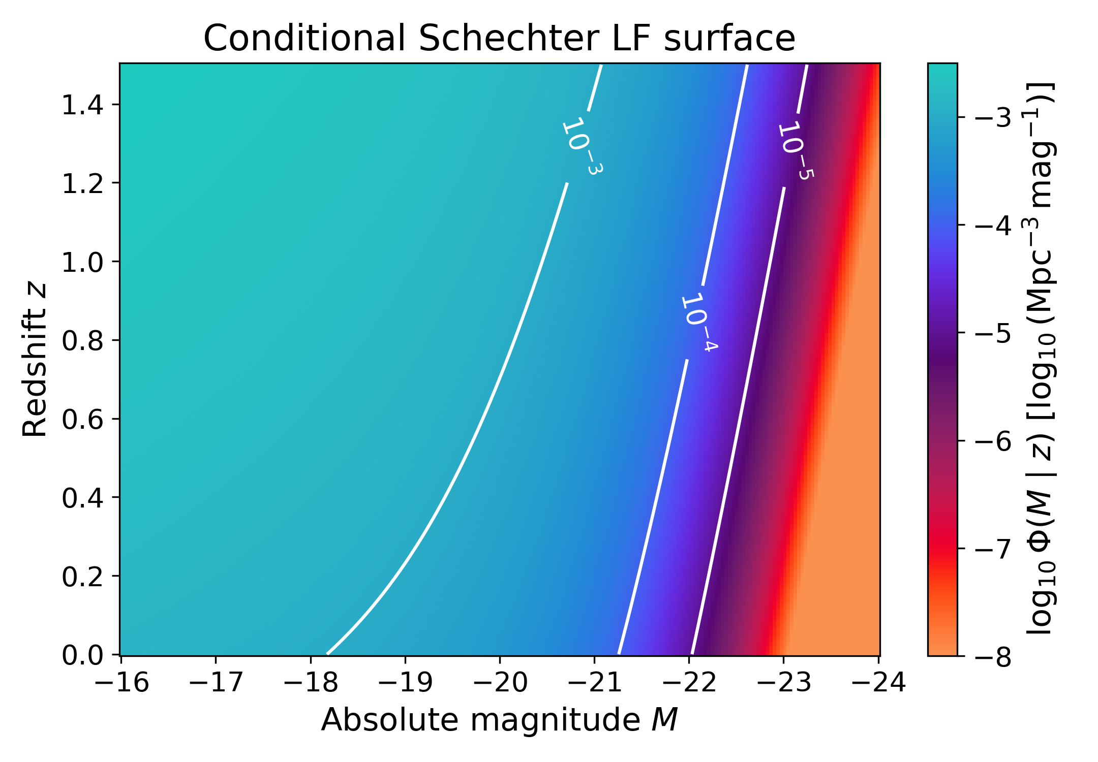
Conditional Schechter surface#
The same conditional luminosity function model can be evaluated over the full magnitude-redshift plane rather than at a few selected redshifts.
The filled colour scale shows \(\log_{10}\Phi(M \mid z)\). The contours mark constant abundance levels. This view is useful for checking the global behaviour of the model: smooth contours indicate that the parameter evolution produces a smooth luminosity function, while abrupt features would signal a problem with the chosen parameterization or redshift dependence.
import numpy as np
import matplotlib.pyplot as plt
import cmasher as cmr

from lfkit import ConditionalLuminosityFunction

LABEL_SIZE = 15
TICK_SIZE = 13
TITLE_SIZE = 17

absolute_mag = np.linspace(-24.0, -16.0, 220)
redshift = np.linspace(0.0, 1.5, 180)

mag_grid, z_grid = np.meshgrid(absolute_mag, redshift)

lf = ConditionalLuminosityFunction.schechter(
    phi_star=lambda z: 1.0e-3 * (1.0 + z) ** 0.8,
    m_star=lambda z: -20.5 - 0.7 * (z - 0.1),
    alpha=-1.1,
)

phi = np.clip(lf.phi(mag_grid, z_grid), 1.0e-8, 1.0e-1)
log_phi = np.log10(phi)

fig, ax = plt.subplots(figsize=(7.2, 5.0))

mesh = ax.pcolormesh(
    absolute_mag,
    redshift,
    log_phi,
    shading="auto",
    cmap="cmr.guppy",
)

contour_levels = [-5.0, -4.0, -3.0, -2.0]
contours = ax.contour(
    absolute_mag,
    redshift,
    log_phi,
    levels=contour_levels,
    colors="white",
    linewidths=1.5,
    linestyles="solid",
)
ax.clabel(contours, inline=True, fontsize=TICK_SIZE, fmt=r"$10^{%.0f}$")

ax.invert_xaxis()
ax.set_xlabel("Absolute magnitude $M$", fontsize=LABEL_SIZE)
ax.set_ylabel("Redshift $z$", fontsize=LABEL_SIZE)
ax.set_title("Conditional Schechter LF surface", fontsize=TITLE_SIZE)
ax.tick_params(axis="both", labelsize=TICK_SIZE)

cbar = fig.colorbar(mesh, ax=ax)
cbar.set_label(
    r"$\log_{10}\Phi(M \mid z)$ "
    r"[$\log_{10}(\mathrm{Mpc}^{-3}\,\mathrm{mag}^{-1})$]",
    fontsize=LABEL_SIZE,
)
cbar.ax.tick_params(labelsize=TICK_SIZE)

plt.tight_layout()
(png)
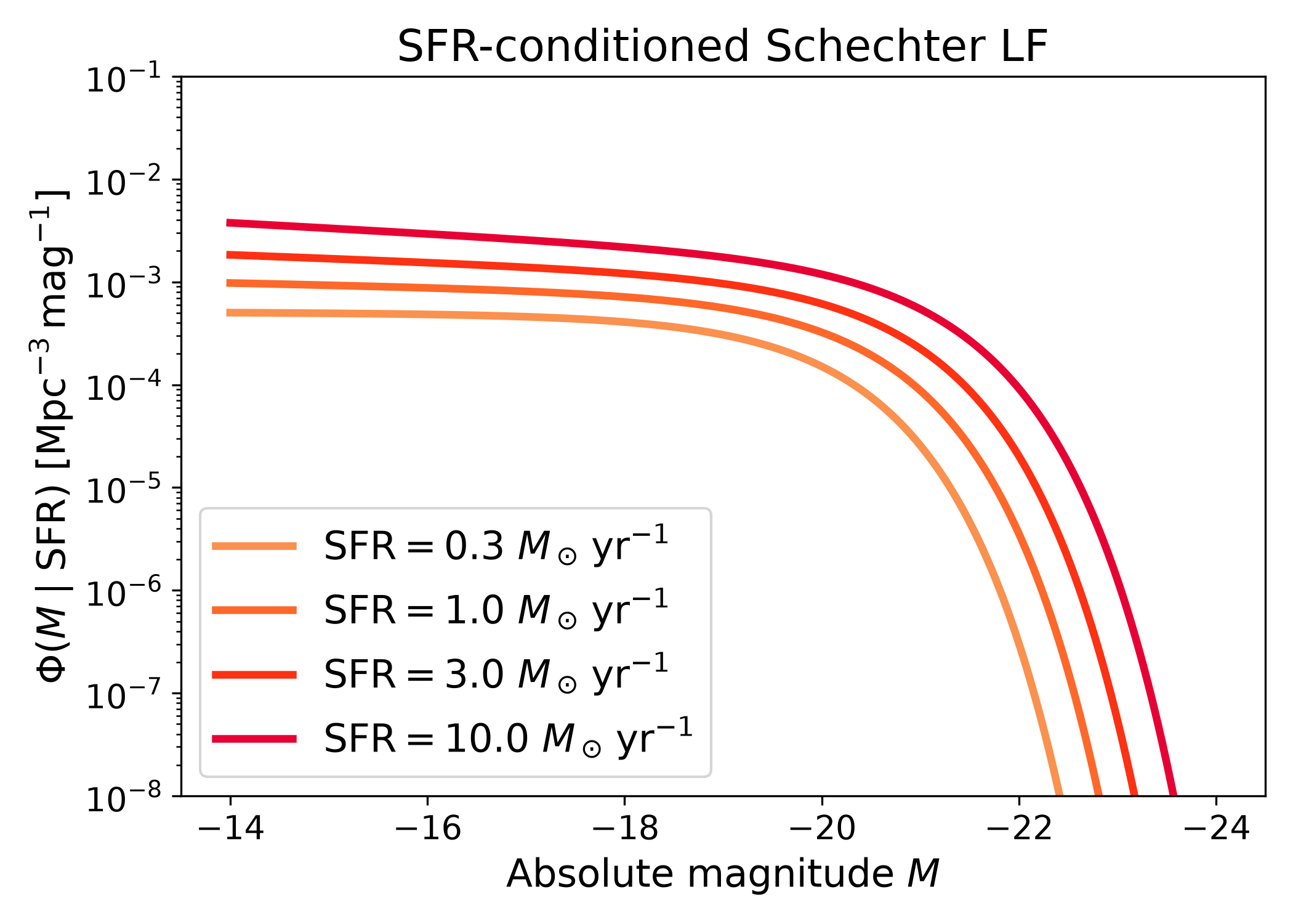
Toy SFR-conditioned Schechter luminosity function#
The conditioning variable does not have to be redshift. The same conditional Schechter API can be used with any external galaxy or environment property. For example, one can write a luminosity function conditioned on star-formation rate,
In this case, each value of sfr selects a different Schechter luminosity
function. The example below is a toy model where galaxies with larger
star-formation rates have a brighter characteristic magnitude and a larger
normalization.
import numpy as np
import matplotlib.pyplot as plt
import cmasher as cmr

from lfkit import ConditionalLuminosityFunction

LABEL_SIZE = 15
TICK_SIZE = 13
TITLE_SIZE = 17
LEGEND_SIZE = 15

absolute_mag = np.linspace(-24.0, -14.0, 500)
sfr_values = [0.3, 1.0, 3.0, 10.0]

colors = cmr.take_cmap_colors(
    "cmr.guppy",
    len(sfr_values),
    cmap_range=(0.0, 0.2),
)

lf = ConditionalLuminosityFunction.schechter(
    phi_star=lambda sfr: 8.0e-4 * (sfr / 1.0) ** 0.35,
    m_star=lambda sfr: -20.2 - 0.7 * np.log10(sfr / 1.0),
    alpha=lambda sfr: -1.05 - 0.08 * np.log10(sfr / 1.0),
)

fig, ax = plt.subplots(figsize=(7.0, 5.0))

for sfr_value, color in zip(sfr_values, colors):
    sfr = np.full_like(absolute_mag, sfr_value)
    phi = lf.phi(absolute_mag, sfr)

    ax.plot(
        absolute_mag,
        phi,
        lw=3,
        color=color,
        label=rf"$\mathrm{{SFR}}={sfr_value}\ M_\odot\,\mathrm{{yr}}^{{-1}}$",
    )

ax.set_yscale("log")
ax.set_ylim(1.0e-8, 1.0e-1)
ax.invert_xaxis()
ax.set_xlabel("Absolute magnitude $M$", fontsize=LABEL_SIZE)
ax.set_ylabel(
    r"$\Phi(M \mid \mathrm{SFR})$ "
    r"[$\mathrm{Mpc}^{-3}\,\mathrm{mag}^{-1}$]",
    fontsize=LABEL_SIZE,
)
ax.set_title("SFR-conditioned Schechter LF", fontsize=TITLE_SIZE)
ax.tick_params(axis="both", labelsize=TICK_SIZE)
ax.legend(frameon=True, fontsize=LEGEND_SIZE, loc="best")

plt.tight_layout()
(png)
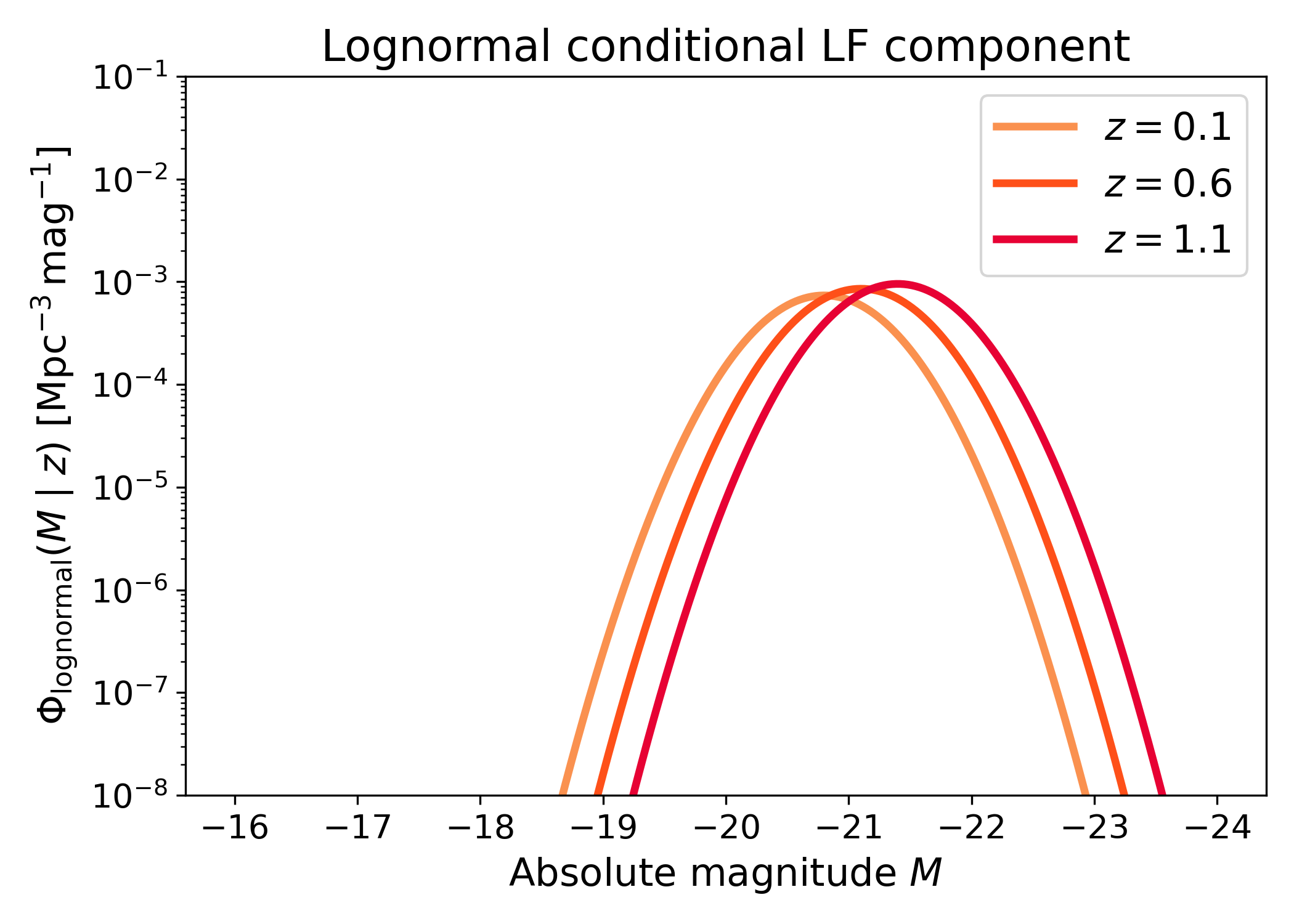
Lognormal conditional component#
A lognormal conditional component describes a population concentrated around a characteristic luminosity at fixed condition. In magnitude space, this appears as a relatively narrow feature centred on a mean absolute magnitude.
This example lets the mean absolute magnitude become brighter with redshift, while the scatter is fixed. The peak therefore shifts to brighter magnitudes as redshift increases, but the width of the component remains similar. This kind of component is useful for representing a population with a preferred luminosity scale rather than a broad Schechter-like faint-end tail.
import numpy as np
import matplotlib.pyplot as plt
import cmasher as cmr

from lfkit import ConditionalLuminosityFunction

LABEL_SIZE = 15
TICK_SIZE = 13
TITLE_SIZE = 17
LEGEND_SIZE = 15

absolute_mag = np.linspace(-24.0, -16.0, 500)
redshifts = [0.1, 0.6, 1.1]

colors = cmr.take_cmap_colors(
    "cmr.guppy",
    len(redshifts),
    cmap_range=(0.0, 0.2),
)

lf = ConditionalLuminosityFunction.lognormal(
    mean_absolute_mag=lambda z: -20.8 - 0.6 * (z - 0.1),
    sigma_log_luminosity=0.18,
    amplitude=lambda z: 8.0e-4 * (1.0 + z) ** 0.4,
)

fig, ax = plt.subplots(figsize=(7.0, 5.0))

for z_value, color in zip(redshifts, colors):
    z = np.full_like(absolute_mag, z_value)
    phi = lf.phi(absolute_mag, z)

    ax.plot(
        absolute_mag,
        phi,
        lw=3,
        color=color,
        label=rf"$z={z_value}$",
    )

ax.set_yscale("log")
ax.set_ylim(1.0e-8, 1.0e-1)
ax.invert_xaxis()
ax.set_xlabel("Absolute magnitude $M$", fontsize=LABEL_SIZE)
ax.set_ylabel(
    r"$\Phi_{\rm lognormal}(M \mid z)$ "
    r"[$\mathrm{Mpc}^{-3}\,\mathrm{mag}^{-1}$]",
    fontsize=LABEL_SIZE,
)
ax.set_title("Lognormal conditional LF component", fontsize=TITLE_SIZE)
ax.tick_params(axis="both", labelsize=TICK_SIZE)
ax.legend(frameon=True, fontsize=LEGEND_SIZE, loc="best")

plt.tight_layout()
(png)
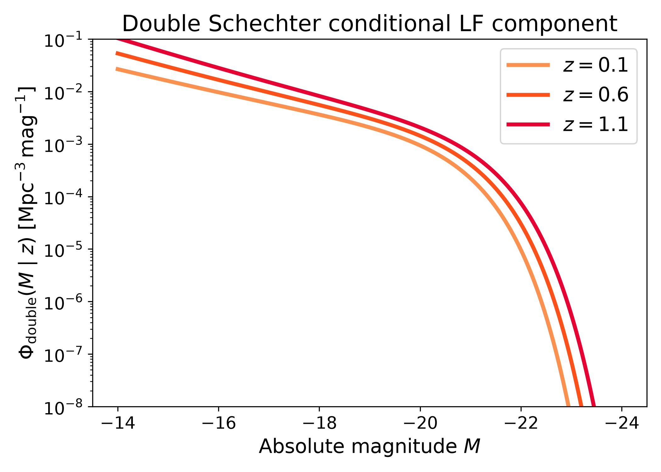
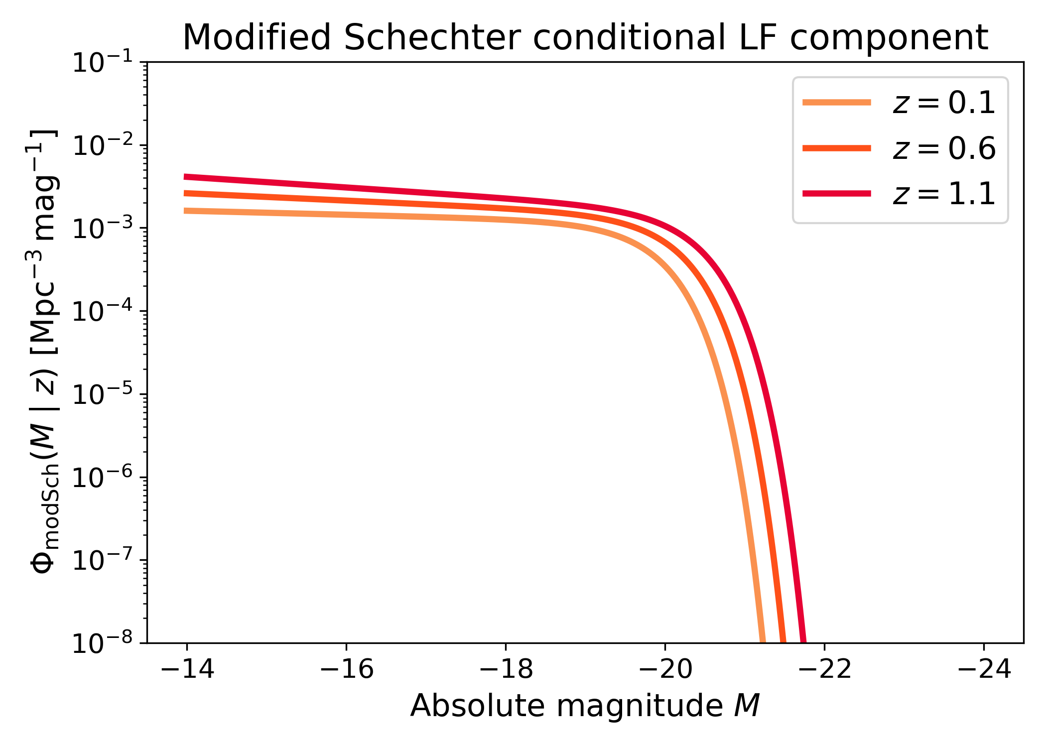
Double Schechter conditional component#
The double Schechter component combines two Schechter-like terms with a shared characteristic magnitude. This gives more flexibility than a single Schechter function because the two components can have different normalizations and faint-end slopes.
This example lets both component normalizations and slopes vary with redshift. The model therefore changes both in amplitude and in shape.
import numpy as np
import matplotlib.pyplot as plt
import cmasher as cmr

from lfkit import ConditionalLuminosityFunction

LABEL_SIZE = 15
TICK_SIZE = 13
TITLE_SIZE = 17
LEGEND_SIZE = 15

absolute_mag = np.linspace(-24.0, -14.0, 500)
redshifts = [0.1, 0.6, 1.1]

colors = cmr.take_cmap_colors(
    "cmr.guppy",
    len(redshifts),
    cmap_range=(0.0, 0.2),
)

lf = ConditionalLuminosityFunction.double_schechter(
    phi_star=lambda z: 1.2e-3 * (1.0 + z) ** 0.5,
    m_star=lambda z: -20.3 - 0.5 * (z - 0.1),
    alpha=lambda z: -1.15 - 0.10 * z,
    beta=lambda z: -0.45 - 0.05 * z,
    m_transition=lambda z: -19.0 - 0.3 * (z - 0.1),
)

fig, ax = plt.subplots(figsize=(7.0, 5.0))

for z_value, color in zip(redshifts, colors):
    z = np.full_like(absolute_mag, z_value)
    phi = lf.phi(absolute_mag, z)
    ax.plot(absolute_mag, phi, lw=3, color=color, label=rf"$z={z_value}$")

ax.set_yscale("log")
ax.set_ylim(1.0e-8, 1.0e-1)
ax.invert_xaxis()
ax.set_xlabel("Absolute magnitude $M$", fontsize=LABEL_SIZE)
ax.set_ylabel(
    r"$\Phi_{\rm double}(M \mid z)$ "
    r"[$\mathrm{Mpc}^{-3}\,\mathrm{mag}^{-1}$]",
    fontsize=LABEL_SIZE,
)
ax.set_title("Double Schechter conditional LF component", fontsize=TITLE_SIZE)
ax.tick_params(axis="both", labelsize=TICK_SIZE)
ax.legend(frameon=True, fontsize=LEGEND_SIZE, loc="best")

plt.tight_layout()
(png)
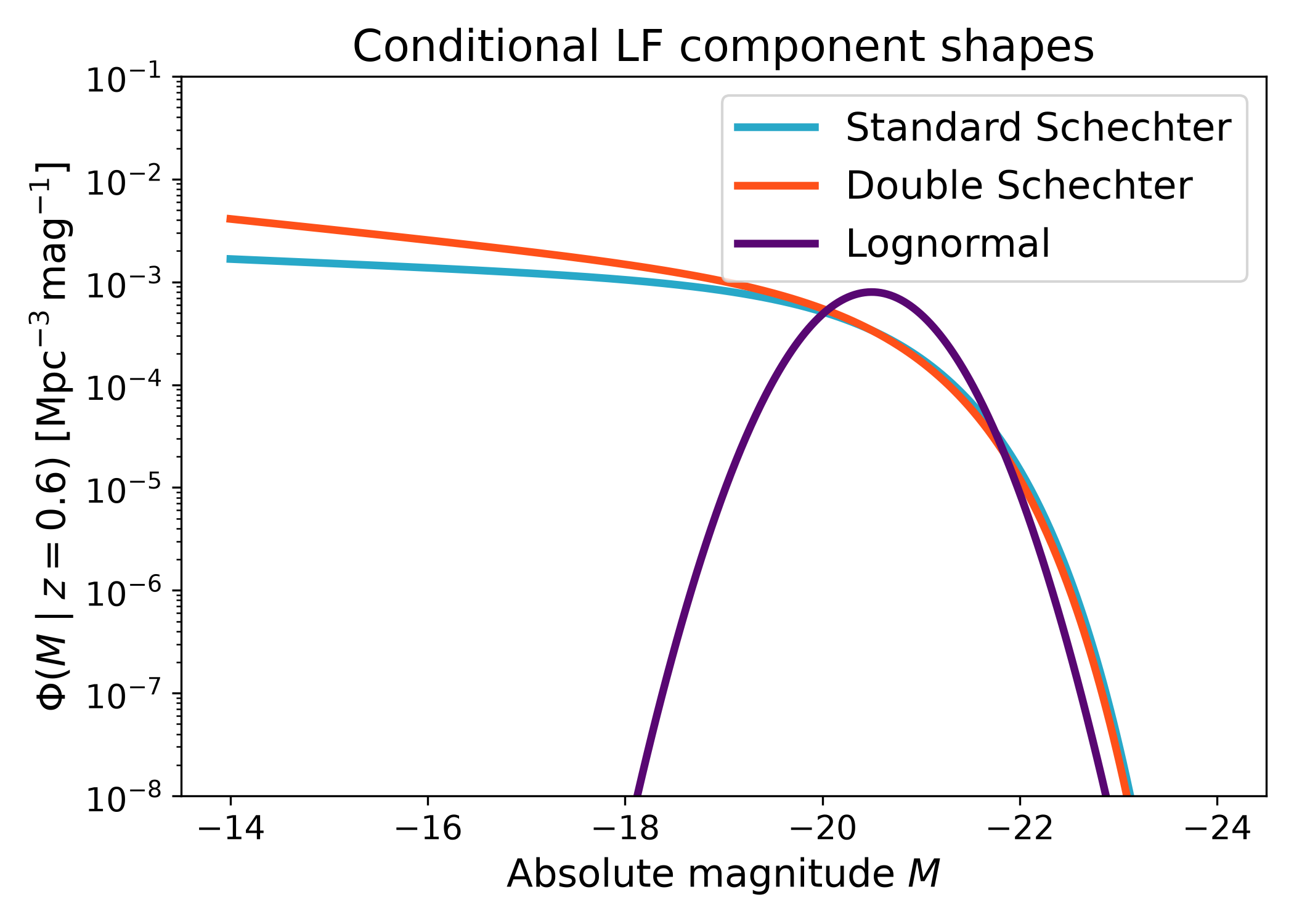
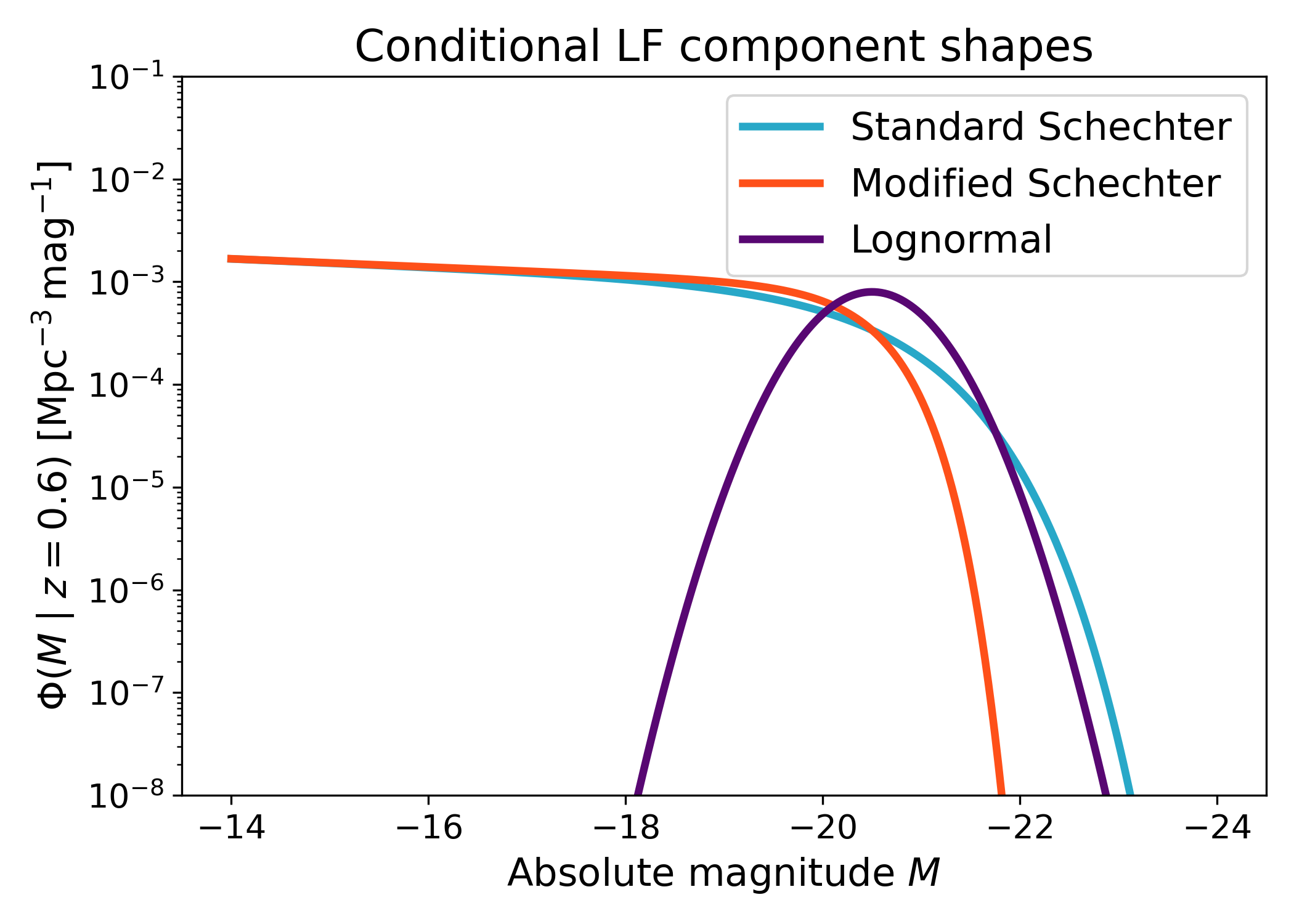
Standard, modified, and lognormal component shapes#
It is useful to compare the component shapes at fixed condition before combining them into more complicated models. This separates differences in functional form from differences caused by redshift or halo-mass evolution.
The standard Schechter form has a power law faint end and an exponential bright-end cutoff. The modified Schechter component has a broader bright-end shape. The lognormal component is localized around a characteristic luminosity. Together, these examples show the kinds of galaxy populations each component is best suited to describe.
import numpy as np
import matplotlib.pyplot as plt
import cmasher as cmr

from lfkit import ConditionalLuminosityFunction

LABEL_SIZE = 15
TICK_SIZE = 13
TITLE_SIZE = 17
LEGEND_SIZE = 15

colors_blue = cmr.take_cmap_colors("cmr.guppy", 3, cmap_range=(0.8, 1.0))
colors_red = cmr.take_cmap_colors("cmr.guppy", 3, cmap_range=(0.0, 0.2))
colors_all = cmr.take_cmap_colors("cmr.guppy", 3, cmap_range=(0.0, 1.0))

absolute_mag = np.linspace(-24.0, -14.0, 600)
z_value = 0.6
z = np.full_like(absolute_mag, z_value)

schechter_lf = ConditionalLuminosityFunction.schechter(
    phi_star=1.0e-3,
    m_star=-20.5,
    alpha=-1.1,
)

modified_lf = ConditionalLuminosityFunction.schechter(
    phi_star=1.0e-3,
    m_star=-20.5,
    alpha=-1.25,
)

lognormal_lf = ConditionalLuminosityFunction.lognormal(
    mean_absolute_mag=-20.5,
    sigma_log_luminosity=0.20,
    amplitude=1.0e-3,
)

phi_schechter = schechter_lf.phi(absolute_mag, z)
phi_modified = modified_lf.phi(absolute_mag, z)
phi_lognormal = lognormal_lf.phi(absolute_mag, z)

fig, ax = plt.subplots(figsize=(7.0, 5.0))

ax.plot(
    absolute_mag,
    phi_schechter,
    lw=3,
    color=colors_blue[1],
    label="Standard Schechter",
)
ax.plot(
    absolute_mag,
    phi_modified,
    lw=3,
    color=colors_red[1],
    label="Double Schechter",
)
ax.plot(
    absolute_mag,
    phi_lognormal,
    lw=3,
    color=colors_all[1],
    label="Lognormal",
)

ax.set_yscale("log")
ax.set_ylim(1.0e-8, 1.0e-1)
ax.invert_xaxis()
ax.set_xlabel("Absolute magnitude $M$", fontsize=LABEL_SIZE)
ax.set_ylabel(
    r"$\Phi(M \mid z=0.6)$ "
    r"[$\mathrm{Mpc}^{-3}\,\mathrm{mag}^{-1}$]",
    fontsize=LABEL_SIZE,
)
ax.set_title("Conditional LF component shapes", fontsize=TITLE_SIZE)
ax.tick_params(axis="both", labelsize=TICK_SIZE)
ax.legend(frameon=True, fontsize=LEGEND_SIZE, loc="best")

plt.tight_layout()
(png)
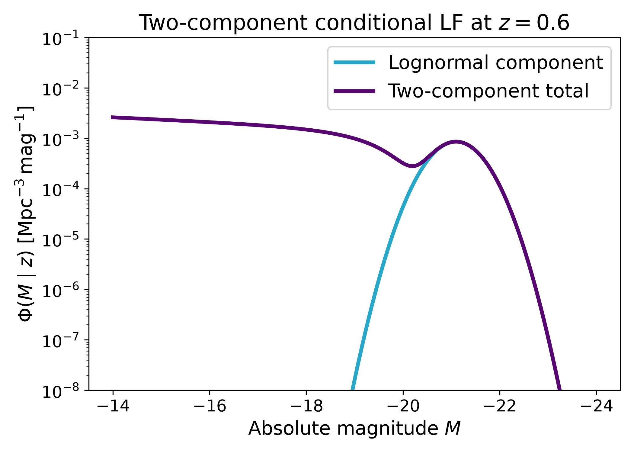
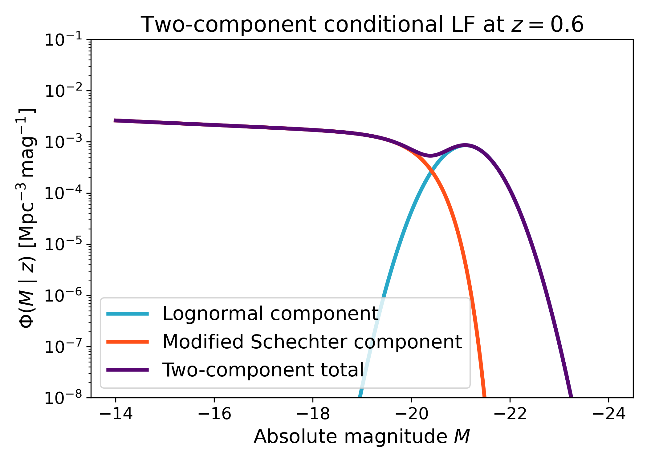
Two-component conditional LF#
The built-in two-component conditional luminosity function combines a lognormal component with a broader Schechter-like component. This is useful when one component is intended to describe a relatively narrow population and the other describes a broader luminosity distribution.
This plot compares the lognormal component with the full two-component model at a fixed redshift. The comparison shows where the narrow component contributes most strongly and where the full model receives additional contribution from the broader component.
import numpy as np
import matplotlib.pyplot as plt
import cmasher as cmr

from lfkit import ConditionalLuminosityFunction

LABEL_SIZE = 15
TICK_SIZE = 13
TITLE_SIZE = 17
LEGEND_SIZE = 15

colors_blue = cmr.take_cmap_colors("cmr.guppy", 3, cmap_range=(0.8, 1.0))
colors_all = cmr.take_cmap_colors("cmr.guppy", 3, cmap_range=(0.0, 1.0))

absolute_mag = np.linspace(-24.0, -14.0, 500)
z_value = 0.6
z = np.full_like(absolute_mag, z_value)

lognormal_lf = ConditionalLuminosityFunction.lognormal(
    mean_absolute_mag=lambda z: -20.8 - 0.6 * (z - 0.1),
    sigma_log_luminosity=0.18,
    amplitude=lambda z: 8.0e-4 * (1.0 + z) ** 0.4,
)

total_lf = ConditionalLuminosityFunction.two_component(
    lognormal_mean_absolute_mag=lambda z: -20.8 - 0.6 * (z - 0.1),
    lognormal_sigma_log_luminosity=0.18,
    lognormal_amplitude=lambda z: 8.0e-4 * (1.0 + z) ** 0.4,
    modified_phi_star=lambda z: 1.2e-3 * (1.0 + z) ** 0.5,
    modified_m_star=lambda z: -19.9 - 0.5 * (z - 0.1),
    modified_alpha=lambda z: -1.05 - 0.10 * z,
)

lognormal_phi = lognormal_lf.phi(absolute_mag, z)
total_phi = total_lf.phi(absolute_mag, z)

fig, ax = plt.subplots(figsize=(7.0, 5.0))

ax.plot(
    absolute_mag,
    lognormal_phi,
    lw=3,
    color=colors_blue[1],
    label="Lognormal component",
)
ax.plot(
    absolute_mag,
    total_phi,
    lw=3,
    color=colors_all[1],
    label="Two-component total",
)

ax.set_yscale("log")
ax.set_ylim(1.0e-8, 1.0e-1)
ax.invert_xaxis()
ax.set_xlabel("Absolute magnitude $M$", fontsize=LABEL_SIZE)
ax.set_ylabel(
    r"$\Phi(M \mid z)$ [$\mathrm{Mpc}^{-3}\,\mathrm{mag}^{-1}$]",
    fontsize=LABEL_SIZE,
)
ax.set_title(r"Two-component conditional LF at $z=0.6$", fontsize=TITLE_SIZE)
ax.tick_params(axis="both", labelsize=TICK_SIZE)
ax.legend(frameon=True, fontsize=LEGEND_SIZE, loc="best")

plt.tight_layout()
(png)
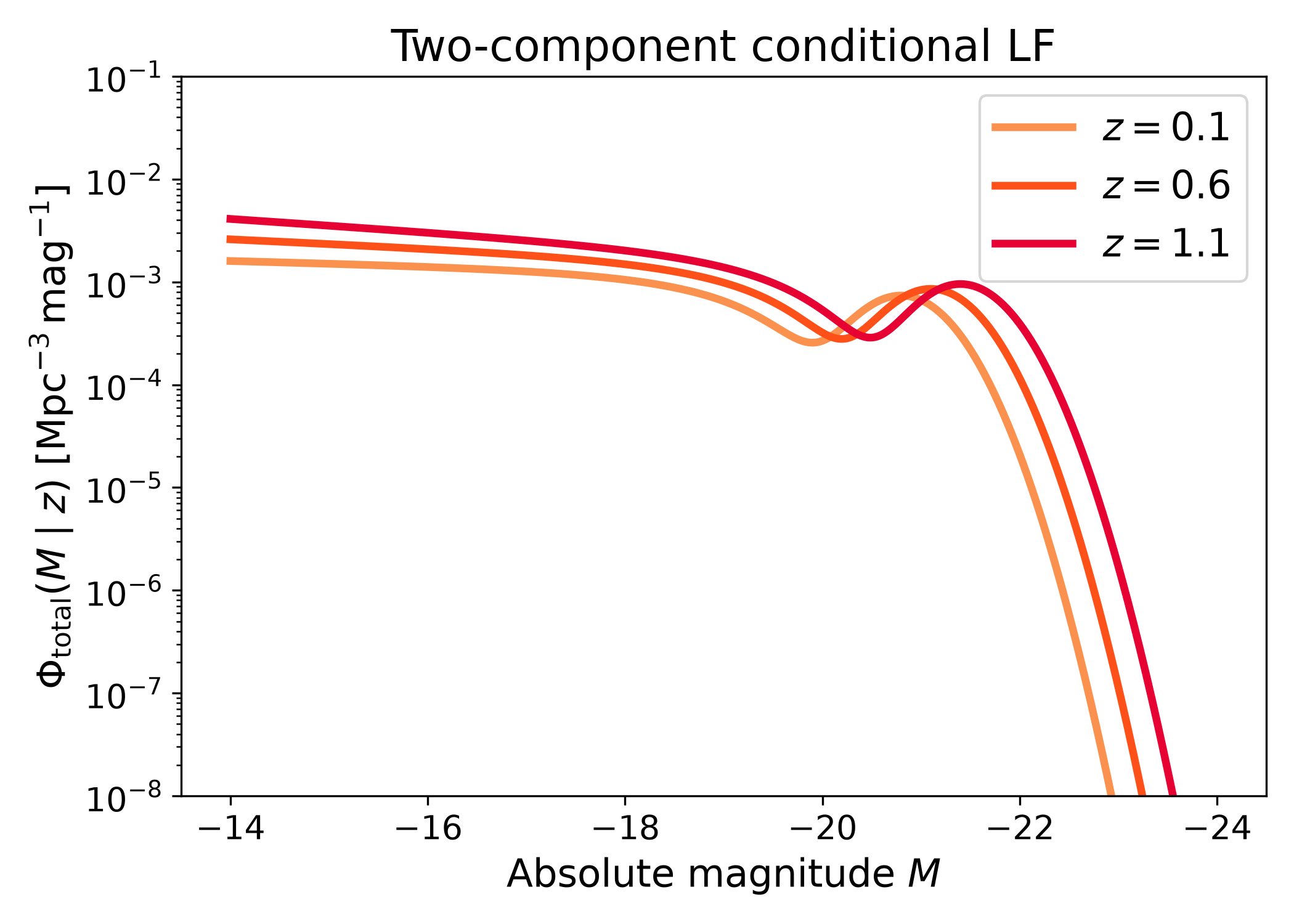
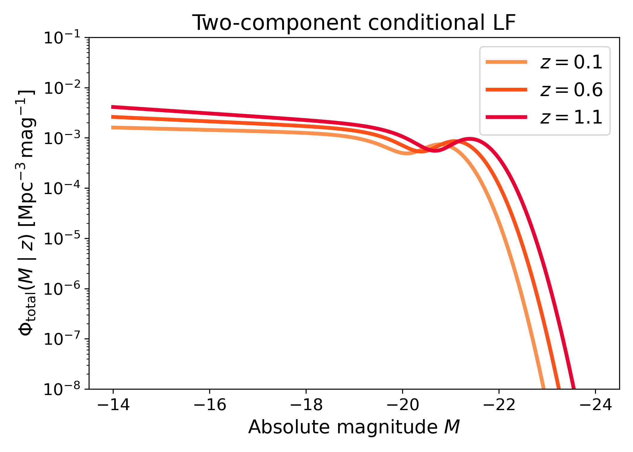
Two-component evolution#
The two-component conditional luminosity function can also be evaluated at several redshifts. This shows how the total population changes when both components depend on the conditioning variable.
Each curve is the sum of the lognormal and modified Schechter components at one redshift. Changes in the curves reflect the combined evolution of the component amplitudes, characteristic magnitudes, and faint-end behaviour. This plot is a compact way to check whether the full conditional model evolves in the expected direction.
import numpy as np
import matplotlib.pyplot as plt
import cmasher as cmr

from lfkit import ConditionalLuminosityFunction

LABEL_SIZE = 15
TICK_SIZE = 13
TITLE_SIZE = 17
LEGEND_SIZE = 15

absolute_mag = np.linspace(-24.0, -14.0, 500)
redshifts = [0.1, 0.6, 1.1]

colors = cmr.take_cmap_colors(
    "cmr.guppy",
    len(redshifts),
    cmap_range=(0.0, 0.2),
)

lf = ConditionalLuminosityFunction.two_component(
    lognormal_mean_absolute_mag=lambda z: -20.8 - 0.6 * (z - 0.1),
    lognormal_sigma_log_luminosity=0.18,
    lognormal_amplitude=lambda z: 8.0e-4 * (1.0 + z) ** 0.4,
    modified_phi_star=lambda z: 1.2e-3 * (1.0 + z) ** 0.5,
    modified_m_star=lambda z: -19.9 - 0.5 * (z - 0.1),
    modified_alpha=lambda z: -1.05 - 0.10 * z,
)

fig, ax = plt.subplots(figsize=(7.0, 5.0))

for z_value, color in zip(redshifts, colors):
    z = np.full_like(absolute_mag, z_value)
    phi = lf.phi(absolute_mag, z)

    ax.plot(
        absolute_mag,
        phi,
        lw=3,
        color=color,
        label=rf"$z={z_value}$",
    )

ax.set_yscale("log")
ax.set_ylim(1.0e-8, 1.0e-1)
ax.invert_xaxis()
ax.set_xlabel("Absolute magnitude $M$", fontsize=LABEL_SIZE)
ax.set_ylabel(
    r"$\Phi_{\rm total}(M \mid z)$ "
    r"[$\mathrm{Mpc}^{-3}\,\mathrm{mag}^{-1}$]",
    fontsize=LABEL_SIZE,
)
ax.set_title("Two-component conditional LF", fontsize=TITLE_SIZE)
ax.tick_params(axis="both", labelsize=TICK_SIZE)
ax.legend(frameon=True, fontsize=LEGEND_SIZE, loc="best")

plt.tight_layout()
(png)
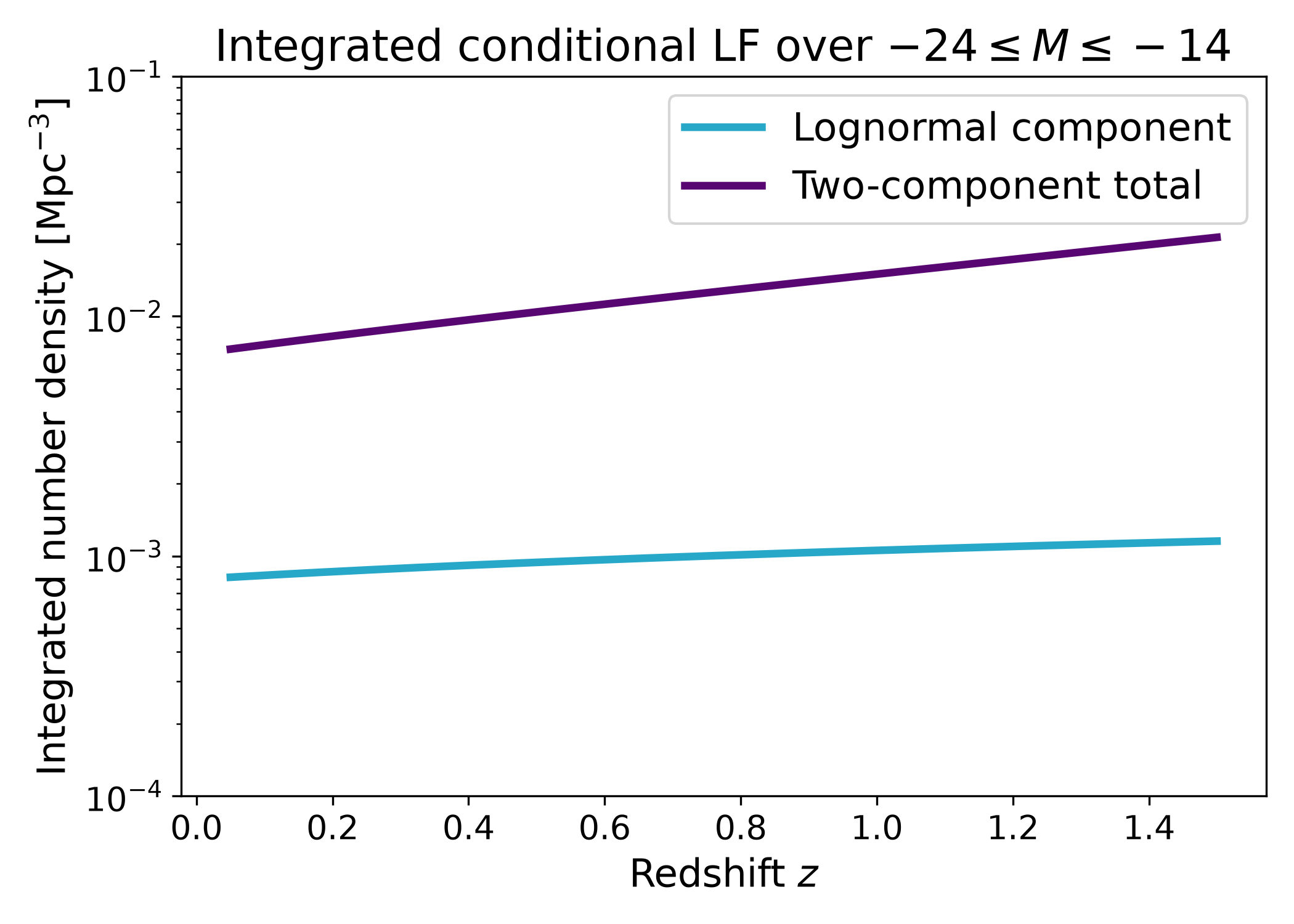
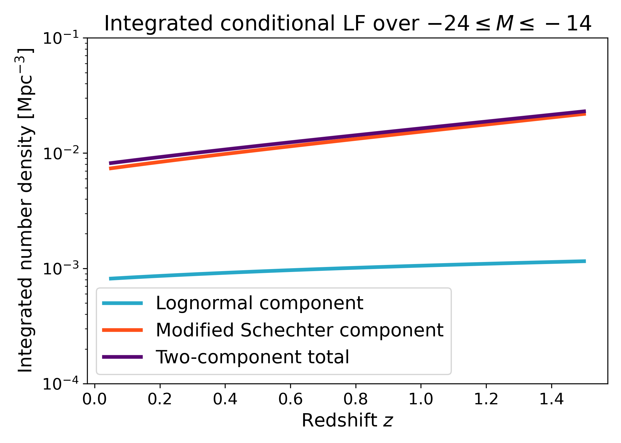
Integrated conditional number density#
A conditional luminosity function can be integrated over absolute magnitude at each value of the conditioning variable. The result is an integrated number density,
For redshift as the conditioning variable, this gives the number density of
galaxies inside the chosen magnitude range as a function of redshift. Because
conditional constructors return normal LFKit luminosity function objects, the
same lf.integrals namespace can be used here.
This example integrates the lognormal component and the full two-component model. The gap between the curves shows the contribution from the broader component in the two-component model.
import numpy as np
import matplotlib.pyplot as plt
import cmasher as cmr

from lfkit import ConditionalLuminosityFunction

LABEL_SIZE = 15
TICK_SIZE = 13
TITLE_SIZE = 17
LEGEND_SIZE = 15

colors_blue = cmr.take_cmap_colors("cmr.guppy", 3, cmap_range=(0.8, 1.0))
colors_all = cmr.take_cmap_colors("cmr.guppy", 3, cmap_range=(0.0, 1.0))

redshift = np.linspace(0.05, 1.5, 180)

lognormal_lf = ConditionalLuminosityFunction.lognormal(
    mean_absolute_mag=lambda z: -20.8 - 0.6 * (z - 0.1),
    sigma_log_luminosity=0.18,
    amplitude=lambda z: 8.0e-4 * (1.0 + z) ** 0.4,
)

total_lf = ConditionalLuminosityFunction.two_component(
    lognormal_mean_absolute_mag=lambda z: -20.8 - 0.6 * (z - 0.1),
    lognormal_sigma_log_luminosity=0.18,
    lognormal_amplitude=lambda z: 8.0e-4 * (1.0 + z) ** 0.4,
    modified_phi_star=lambda z: 1.2e-3 * (1.0 + z) ** 0.5,
    modified_m_star=lambda z: -19.9 - 0.5 * (z - 0.1),
    modified_alpha=lambda z: -1.05 - 0.10 * z,
)

n_lognormal = lognormal_lf.integrals.number_density(
    redshift,
    m_bright=-24.0,
    m_faint=-14.0,
    n_m=800,
)

n_total = total_lf.integrals.number_density(
    redshift,
    m_bright=-24.0,
    m_faint=-14.0,
    n_m=800,
)

fig, ax = plt.subplots(figsize=(7.0, 5.0))

ax.plot(
    redshift,
    n_lognormal,
    lw=3,
    color=colors_blue[1],
    label="Lognormal component",
)
ax.plot(
    redshift,
    n_total,
    lw=3,
    color=colors_all[1],
    label="Two-component total",
)

ax.set_yscale("log")
ax.set_ylim(1.0e-4, 1.0e-1)
ax.set_xlabel("Redshift $z$", fontsize=LABEL_SIZE)
ax.set_ylabel(r"Integrated number density [$\mathrm{Mpc}^{-3}$]", fontsize=LABEL_SIZE)
ax.set_title(r"Integrated conditional LF over $-24 \leq M \leq -14$", fontsize=TITLE_SIZE)
ax.tick_params(axis="both", labelsize=TICK_SIZE)
ax.legend(frameon=True, fontsize=LEGEND_SIZE, loc="best")

plt.tight_layout()
(png)
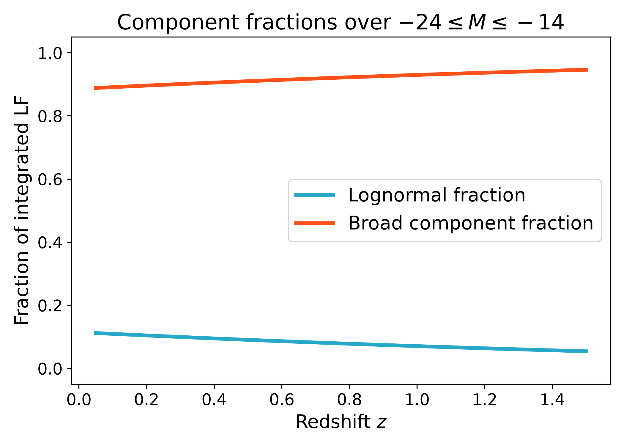
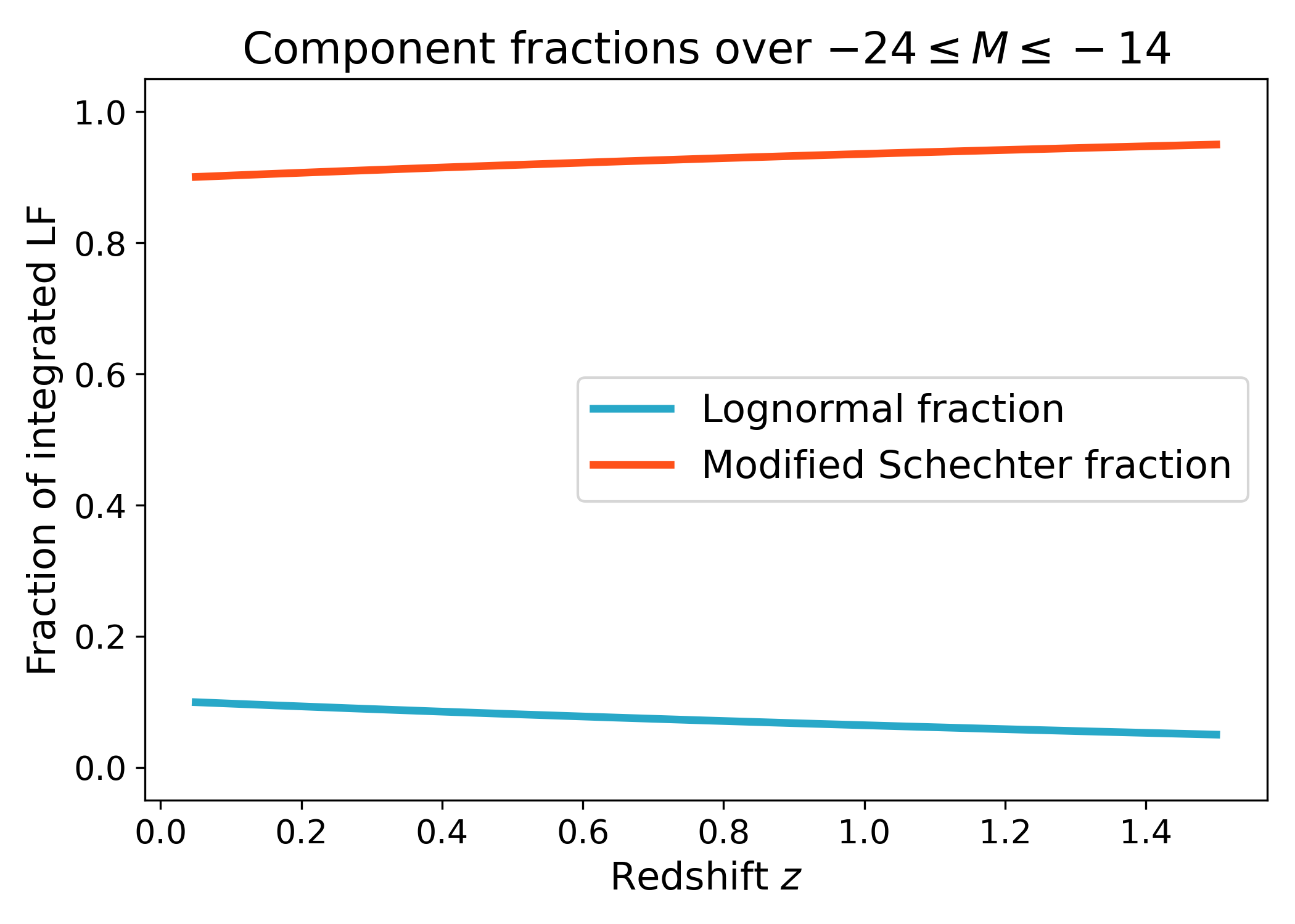
Component fractions#
The relative contribution of the lognormal component can be summarized as a fraction of the integrated two-component luminosity function,
The remaining fraction is the contribution from the broader component in the two-component model. This is often easier to interpret than comparing raw number densities alone.
import numpy as np
import matplotlib.pyplot as plt
import cmasher as cmr

from lfkit import ConditionalLuminosityFunction

LABEL_SIZE = 15
TICK_SIZE = 13
TITLE_SIZE = 17
LEGEND_SIZE = 15

colors_blue = cmr.take_cmap_colors("cmr.guppy", 3, cmap_range=(0.8, 1.0))
colors_red = cmr.take_cmap_colors("cmr.guppy", 3, cmap_range=(0.0, 0.2))

redshift = np.linspace(0.05, 1.5, 180)

lognormal_lf = ConditionalLuminosityFunction.lognormal(
    mean_absolute_mag=lambda z: -20.8 - 0.6 * (z - 0.1),
    sigma_log_luminosity=0.18,
    amplitude=lambda z: 8.0e-4 * (1.0 + z) ** 0.4,
)

total_lf = ConditionalLuminosityFunction.two_component(
    lognormal_mean_absolute_mag=lambda z: -20.8 - 0.6 * (z - 0.1),
    lognormal_sigma_log_luminosity=0.18,
    lognormal_amplitude=lambda z: 8.0e-4 * (1.0 + z) ** 0.4,
    modified_phi_star=lambda z: 1.2e-3 * (1.0 + z) ** 0.5,
    modified_m_star=lambda z: -19.9 - 0.5 * (z - 0.1),
    modified_alpha=lambda z: -1.05 - 0.10 * z,
)

n_lognormal = lognormal_lf.integrals.number_density(
    redshift,
    m_bright=-24.0,
    m_faint=-14.0,
    n_m=800,
)

n_total = total_lf.integrals.number_density(
    redshift,
    m_bright=-24.0,
    m_faint=-14.0,
    n_m=800,
)

lognormal_fraction = n_lognormal / n_total
broad_fraction = 1.0 - lognormal_fraction

fig, ax = plt.subplots(figsize=(7.0, 5.0))

ax.plot(
    redshift,
    lognormal_fraction,
    lw=3,
    color=colors_blue[1],
    label="Lognormal fraction",
)
ax.plot(
    redshift,
    broad_fraction,
    lw=3,
    color=colors_red[1],
    label="Broad component fraction",
)

ax.set_ylim(-0.05, 1.05)
ax.set_xlabel("Redshift $z$", fontsize=LABEL_SIZE)
ax.set_ylabel("Fraction of integrated LF", fontsize=LABEL_SIZE)
ax.set_title(r"Component fractions over $-24 \leq M \leq -14$", fontsize=TITLE_SIZE)
ax.tick_params(axis="both", labelsize=TICK_SIZE)
ax.legend(frameon=True, fontsize=LEGEND_SIZE, loc="center right")

plt.tight_layout()
(png)
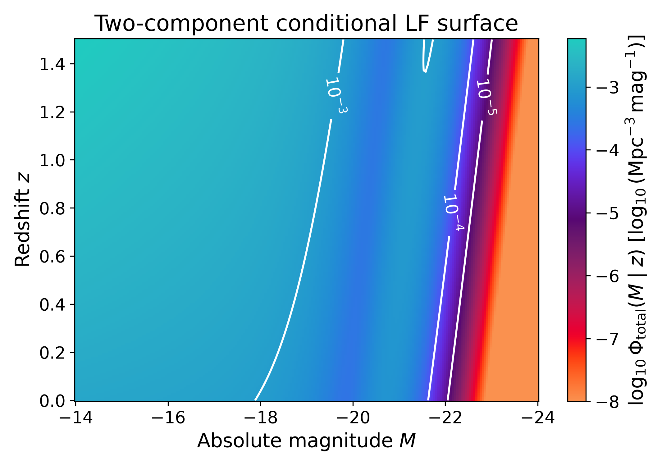
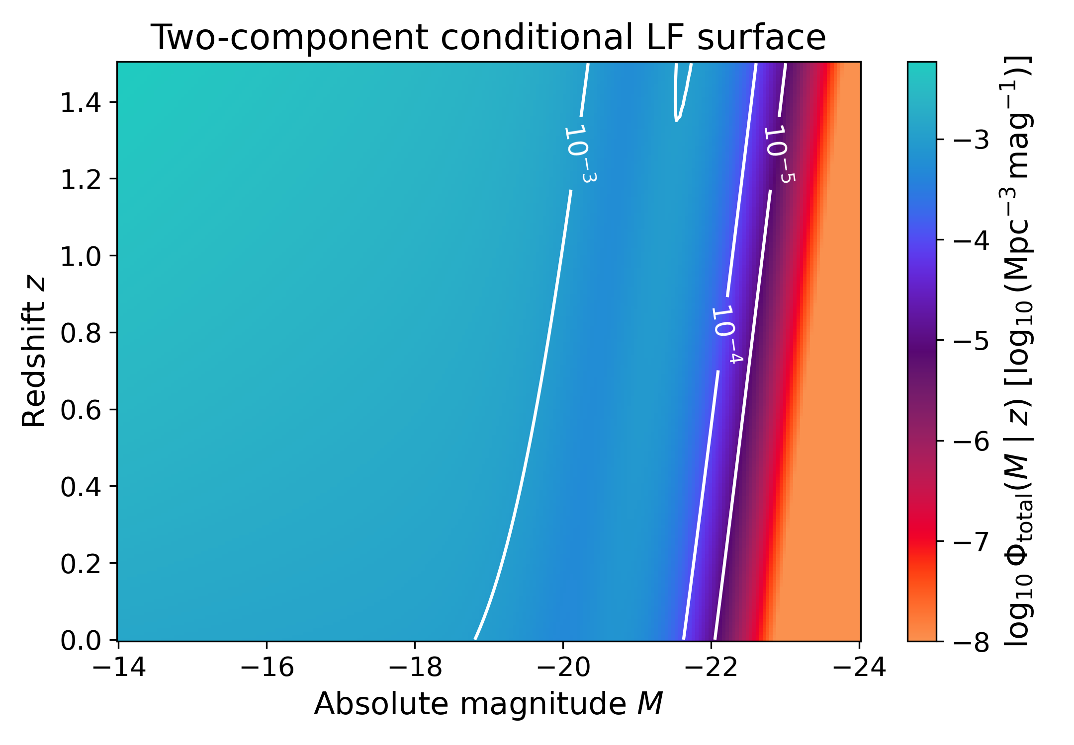
Two-component LF surface#
The full two-component conditional luminosity function can be shown as a surface in the magnitude-redshift plane. This combines the component structure and the redshift evolution in a single diagnostic plot.
The filled colour scale shows \(\log_{10}\Phi_{\rm total}(M \mid z)\). The contours mark constant abundance levels. This view is useful for checking whether the narrow component, broad component, and redshift dependence combine smoothly across the full domain. It also makes it easier to identify where the model predicts the largest abundance of galaxies.
import numpy as np
import matplotlib.pyplot as plt
import cmasher as cmr

from lfkit import ConditionalLuminosityFunction

LABEL_SIZE = 15
TICK_SIZE = 13
TITLE_SIZE = 17

absolute_mag = np.linspace(-24.0, -14.0, 220)
redshift = np.linspace(0.0, 1.5, 180)

mag_grid, z_grid = np.meshgrid(absolute_mag, redshift)

lf = ConditionalLuminosityFunction.two_component(
    lognormal_mean_absolute_mag=lambda z: -20.8 - 0.6 * (z - 0.1),
    lognormal_sigma_log_luminosity=0.18,
    lognormal_amplitude=lambda z: 8.0e-4 * (1.0 + z) ** 0.4,
    modified_phi_star=lambda z: 1.2e-3 * (1.0 + z) ** 0.5,
    modified_m_star=lambda z: -19.9 - 0.5 * (z - 0.1),
    modified_alpha=lambda z: -1.05 - 0.10 * z,
)

phi = np.clip(lf.phi(mag_grid, z_grid), 1.0e-8, 1.0e-1)
log_phi = np.log10(phi)

fig, ax = plt.subplots(figsize=(7.2, 5.0))

mesh = ax.pcolormesh(
    absolute_mag,
    redshift,
    log_phi,
    shading="auto",
    cmap="cmr.guppy",
)

contour_levels = [-5.0, -4.0, -3.0, -2.0]
contours = ax.contour(
    absolute_mag,
    redshift,
    log_phi,
    levels=contour_levels,
    colors="white",
    linewidths=1.5,
    linestyles="solid",
)
ax.clabel(contours, inline=True, fontsize=TICK_SIZE, fmt=r"$10^{%.0f}$")

ax.invert_xaxis()
ax.set_xlabel("Absolute magnitude $M$", fontsize=LABEL_SIZE)
ax.set_ylabel("Redshift $z$", fontsize=LABEL_SIZE)
ax.set_title("Two-component conditional LF surface", fontsize=TITLE_SIZE)
ax.tick_params(axis="both", labelsize=TICK_SIZE)

cbar = fig.colorbar(mesh, ax=ax)
cbar.set_label(
    r"$\log_{10}\Phi_{\rm total}(M \mid z)$ "
    r"[$\log_{10}(\mathrm{Mpc}^{-3}\,\mathrm{mag}^{-1})$]",
    fontsize=LABEL_SIZE,
)
cbar.ax.tick_params(labelsize=TICK_SIZE)

plt.tight_layout()
(png)
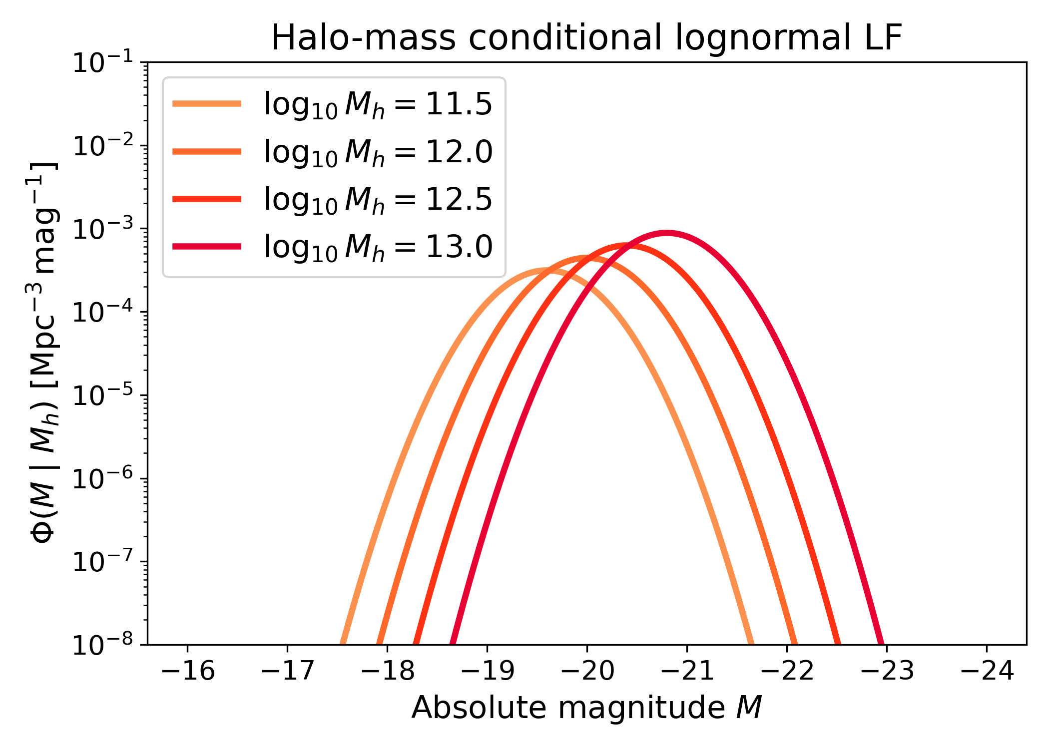
Halo-mass conditional luminosity function#
The conditioning variable does not need to be redshift. In halo-model applications, a conditional luminosity function is often written as \(\Phi(M \mid M_h)\), where \(M_h\) is halo mass. This describes the luminosity distribution of galaxies hosted by halos of a given mass.
This example uses log halo mass as the conditioning variable. The lognormal mean magnitude becomes brighter in more massive halos, and the amplitude also increases with halo mass. The interpretation is that more massive halos host brighter and more abundant galaxies in this toy model.
import numpy as np
import matplotlib.pyplot as plt
import cmasher as cmr

from lfkit import ConditionalLuminosityFunction

LABEL_SIZE = 15
TICK_SIZE = 13
TITLE_SIZE = 17
LEGEND_SIZE = 15

absolute_mag = np.linspace(-24.0, -16.0, 600)
log_halo_masses = [11.5, 12.0, 12.5, 13.0]

colors = cmr.take_cmap_colors(
    "cmr.guppy",
    len(log_halo_masses),
    cmap_range=(0.0, 0.2),
)

lf = ConditionalLuminosityFunction.lognormal(
    mean_absolute_mag=lambda log_mh: -20.0 - 0.8 * (log_mh - 12.0),
    sigma_log_luminosity=0.18,
    amplitude=lambda log_mh: 5.0e-4 * 10.0 ** (0.3 * (log_mh - 12.0)),
)

fig, ax = plt.subplots(figsize=(7.0, 5.0))

for log_mh, color in zip(log_halo_masses, colors):
    condition = np.full_like(absolute_mag, log_mh)
    phi = lf.phi(absolute_mag, condition)

    ax.plot(
        absolute_mag,
        phi,
        lw=3,
        color=color,
        label=rf"$\log_{{10}} M_h={log_mh}$",
    )

ax.set_yscale("log")
ax.set_ylim(1.0e-8, 1.0e-1)
ax.invert_xaxis()
ax.set_xlabel("Absolute magnitude $M$", fontsize=LABEL_SIZE)
ax.set_ylabel(
    r"$\Phi(M \mid M_h)$ [$\mathrm{Mpc}^{-3}\,\mathrm{mag}^{-1}$]",
    fontsize=LABEL_SIZE,
)
ax.set_title("Halo-mass conditional lognormal LF", fontsize=TITLE_SIZE)
ax.tick_params(axis="both", labelsize=TICK_SIZE)
ax.legend(frameon=True, fontsize=LEGEND_SIZE, loc="best")

plt.tight_layout()
(png)
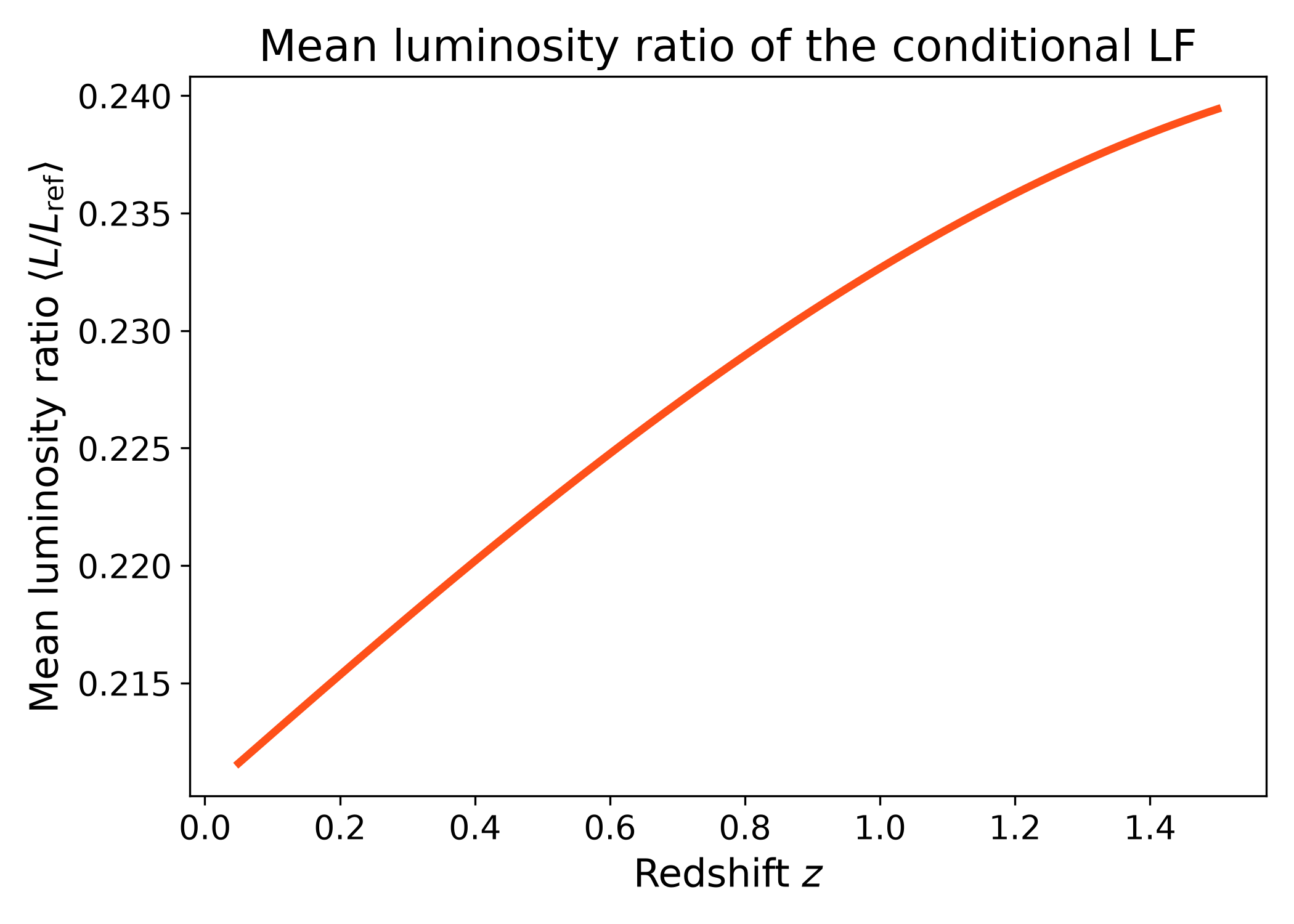
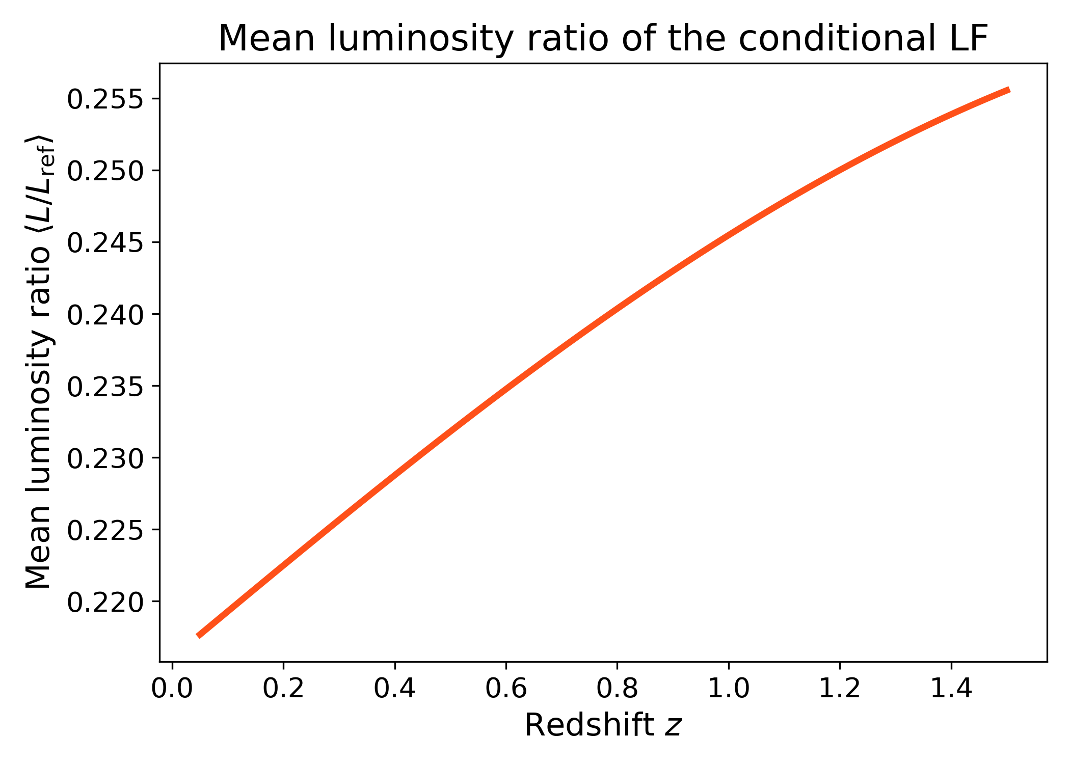
Mean luminosity ratio from a conditional luminosity function#
Weighted integrals can be used to compute luminosity-weighted summary statistics of a conditional luminosity function. Instead of only counting galaxies, the integral can weight each magnitude by a physically meaningful quantity.
For example, the mean luminosity ratio relative to a reference magnitude is
This example uses the lf.integrals namespace on a two-component conditional
luminosity function. The numerator is a luminosity-weighted integral and the
denominator is the number density. Their ratio gives the average luminosity of
the selected population relative to the chosen reference luminosity.
import numpy as np
import matplotlib.pyplot as plt
import cmasher as cmr

from lfkit import ConditionalLuminosityFunction

LABEL_SIZE = 15
TICK_SIZE = 13
TITLE_SIZE = 17

redshift = np.linspace(0.05, 1.5, 180)
reference_mag = -20.5

lf = ConditionalLuminosityFunction.two_component(
    lognormal_mean_absolute_mag=lambda z: -20.8 - 0.6 * (z - 0.1),
    lognormal_sigma_log_luminosity=0.18,
    lognormal_amplitude=lambda z: 8.0e-4 * (1.0 + z) ** 0.4,
    modified_phi_star=lambda z: 1.2e-3 * (1.0 + z) ** 0.5,
    modified_m_star=lambda z: -19.9 - 0.5 * (z - 0.1),
    modified_alpha=lambda z: -1.05 - 0.10 * z,
)

number_density = lf.integrals.number_density(
    redshift,
    m_bright=-24.0,
    m_faint=-14.0,
    n_m=800,
)

weighted_luminosity_ratio = lf.integrals.weighted(
    redshift,
    weight_fn=lambda absolute_mag, condition: 10.0 ** (
        -0.4 * (absolute_mag - reference_mag)
    ),
    m_bright=-24.0,
    m_faint=-14.0,
    n_m=800,
)

mean_luminosity_ratio = weighted_luminosity_ratio / number_density

fig, ax = plt.subplots(figsize=(7.0, 5.0))

ax.plot(
    redshift,
    mean_luminosity_ratio,
    lw=3,
    color=cmr.take_cmap_colors("cmr.guppy", 3, cmap_range=(0.0, 0.2))[1],
)

ax.set_xlabel("Redshift $z$", fontsize=LABEL_SIZE)
ax.set_ylabel(r"Mean luminosity ratio $\langle L/L_{\rm ref} \rangle$", fontsize=LABEL_SIZE)
ax.set_title("Mean luminosity ratio of the conditional LF", fontsize=TITLE_SIZE)
ax.tick_params(axis="both", labelsize=TICK_SIZE)

plt.tight_layout()
(png)
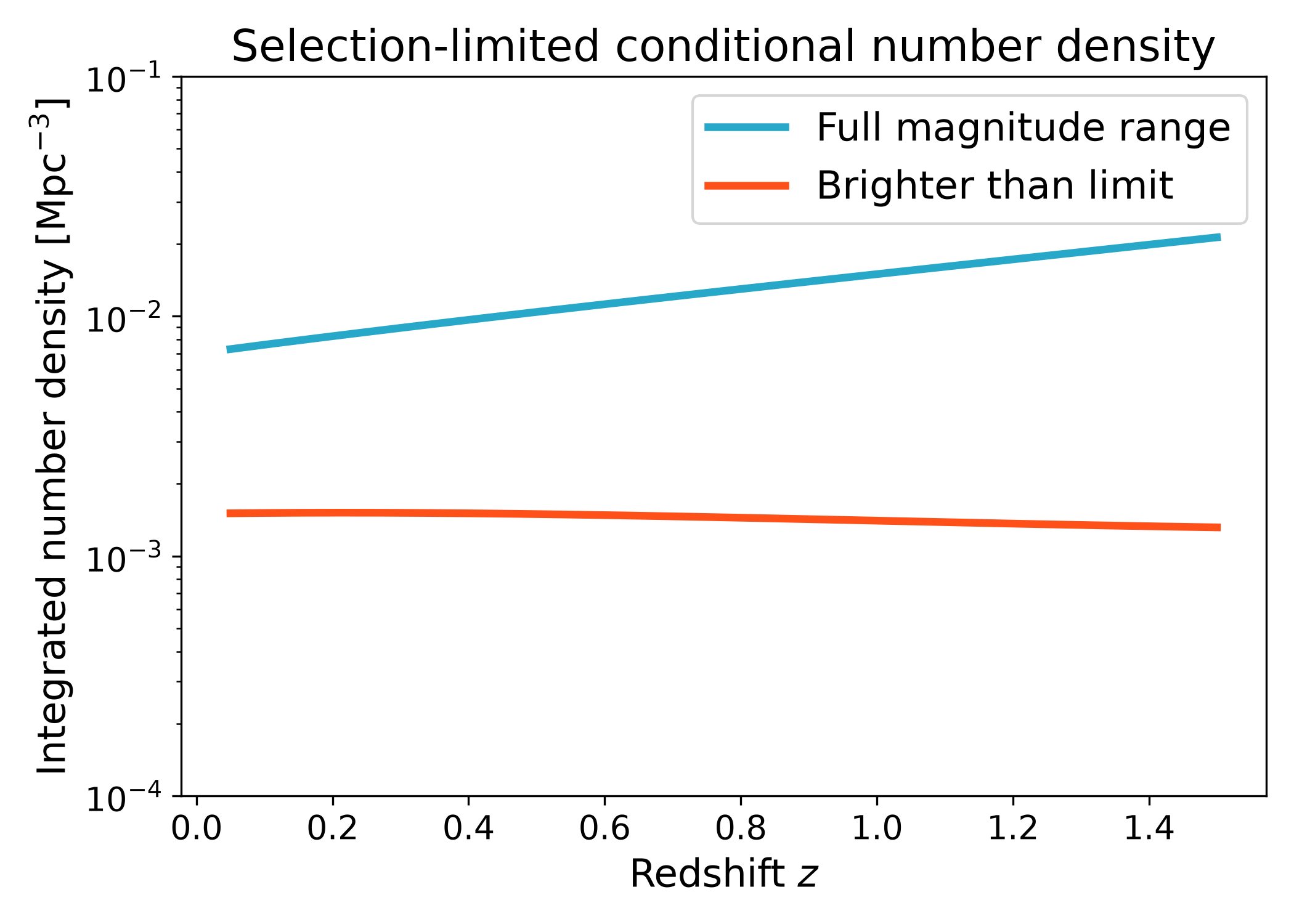
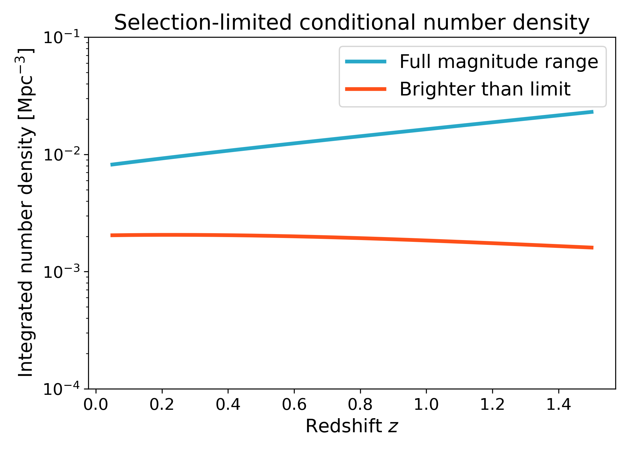
Selection-limited conditional number density#
The LFKit API can integrate a conditional luminosity function over finite magnitude bounds. This is useful for survey-like selections where only galaxies brighter than a limiting absolute magnitude contribute to the observed sample.
Here, the limiting absolute magnitude becomes brighter with redshift. The example compares the full number density over a fixed reference magnitude range with the number density brighter than the redshift-dependent limit. The gap between the two curves shows how much of the luminosity function is excluded by the selection.
import numpy as np
import matplotlib.pyplot as plt
import cmasher as cmr

from lfkit import ConditionalLuminosityFunction

LABEL_SIZE = 15
TICK_SIZE = 13
TITLE_SIZE = 17
LEGEND_SIZE = 15

redshift = np.linspace(0.05, 1.5, 180)

lf = ConditionalLuminosityFunction.two_component(
    lognormal_mean_absolute_mag=lambda z: -20.8 - 0.6 * (z - 0.1),
    lognormal_sigma_log_luminosity=0.18,
    lognormal_amplitude=lambda z: 8.0e-4 * (1.0 + z) ** 0.4,
    modified_phi_star=lambda z: 1.2e-3 * (1.0 + z) ** 0.5,
    modified_m_star=lambda z: -19.9 - 0.5 * (z - 0.1),
    modified_alpha=lambda z: -1.05 - 0.10 * z,
)

limiting_mag = -18.5 - 1.2 * redshift

n_total = lf.integrals.number_density(
    redshift,
    m_bright=-24.0,
    m_faint=-14.0,
    n_m=800,
)

n_selected = lf.integrals.number_density(
    redshift,
    m_bright=-24.0,
    m_faint=limiting_mag,
    n_m=800,
)

colors_blue = cmr.take_cmap_colors("cmr.guppy", 3, cmap_range=(0.8, 1.0))
colors_red = cmr.take_cmap_colors("cmr.guppy", 3, cmap_range=(0.0, 0.2))

fig, ax = plt.subplots(figsize=(7.0, 5.0))

ax.plot(
    redshift,
    n_total,
    lw=3,
    color=colors_blue[1],
    label="Full magnitude range",
)
ax.plot(
    redshift,
    n_selected,
    lw=3,
    color=colors_red[1],
    label="Brighter than limit",
)

ax.set_yscale("log")
ax.set_ylim(1.0e-4, 1.0e-1)
ax.set_xlabel("Redshift $z$", fontsize=LABEL_SIZE)
ax.set_ylabel(
    r"Integrated number density [$\mathrm{Mpc}^{-3}$]",
    fontsize=LABEL_SIZE,
)
ax.set_title("Selection-limited conditional number density", fontsize=TITLE_SIZE)
ax.tick_params(axis="both", labelsize=TICK_SIZE)
ax.legend(frameon=True, fontsize=LEGEND_SIZE, loc="best")

plt.tight_layout()
(png)
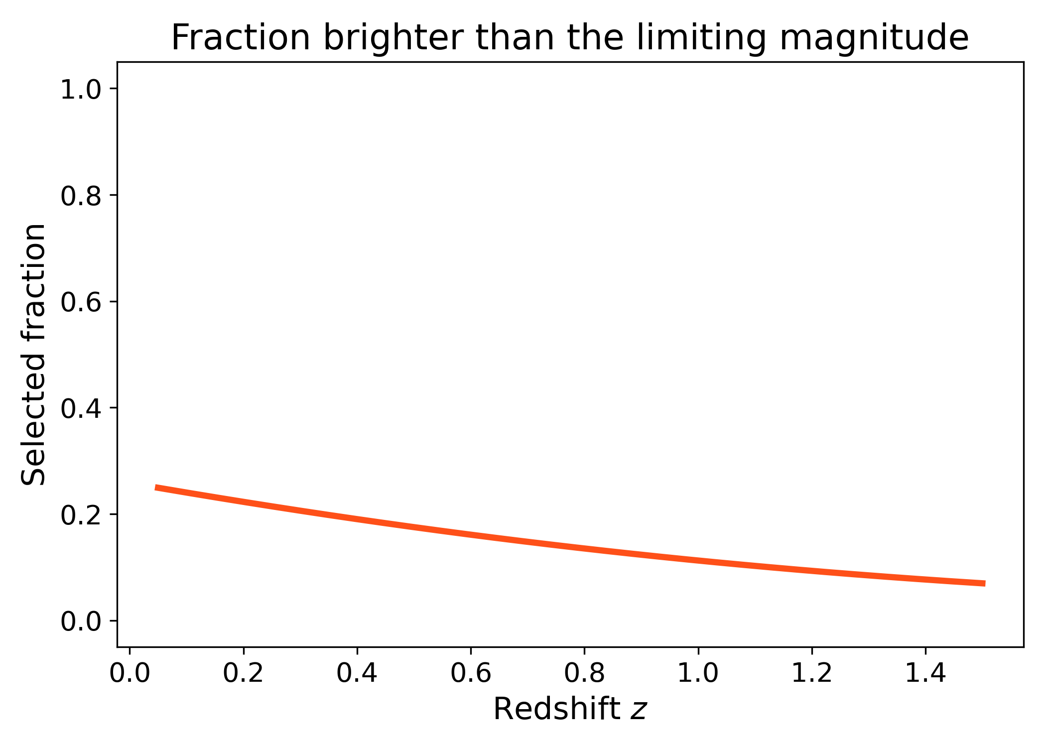
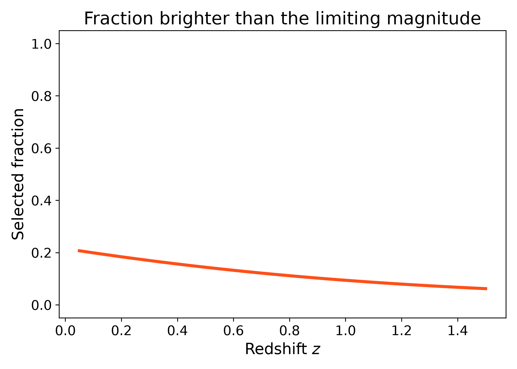
Selection fraction#
The selected fraction is the ratio between the number density brighter than the redshift-dependent limiting magnitude and the number density over the full reference magnitude range,
This diagnostic compresses the selection effect into a number between zero and one. Values close to one mean that most of the reference luminosity function is included by the selection. Smaller values mean that the limiting magnitude removes a larger fraction of the population.
import numpy as np
import matplotlib.pyplot as plt
import cmasher as cmr

from lfkit import ConditionalLuminosityFunction

LABEL_SIZE = 15
TICK_SIZE = 13
TITLE_SIZE = 17

redshift = np.linspace(0.05, 1.5, 180)

lf = ConditionalLuminosityFunction.two_component(
    lognormal_mean_absolute_mag=lambda z: -20.8 - 0.6 * (z - 0.1),
    lognormal_sigma_log_luminosity=0.18,
    lognormal_amplitude=lambda z: 8.0e-4 * (1.0 + z) ** 0.4,
    modified_phi_star=lambda z: 1.2e-3 * (1.0 + z) ** 0.5,
    modified_m_star=lambda z: -19.9 - 0.5 * (z - 0.1),
    modified_alpha=lambda z: -1.05 - 0.10 * z,
)

limiting_mag = -18.5 - 1.2 * redshift

n_total = lf.integrals.number_density(
    redshift,
    m_bright=-24.0,
    m_faint=-14.0,
    n_m=800,
)

n_selected = lf.integrals.number_density(
    redshift,
    m_bright=-24.0,
    m_faint=limiting_mag,
    n_m=800,
)

selected_fraction = n_selected / n_total

color = cmr.take_cmap_colors("cmr.guppy", 3, cmap_range=(0.0, 0.2))[1]

fig, ax = plt.subplots(figsize=(7.0, 5.0))

ax.plot(redshift, selected_fraction, lw=3, color=color)

ax.set_ylim(-0.05, 1.05)
ax.set_xlabel("Redshift $z$", fontsize=LABEL_SIZE)
ax.set_ylabel("Selected fraction", fontsize=LABEL_SIZE)
ax.set_title("Fraction brighter than the limiting magnitude", fontsize=TITLE_SIZE)
ax.tick_params(axis="both", labelsize=TICK_SIZE)

plt.tight_layout()
(png)