kcorrect examples#
This page provides basic, executable examples showing how to use
lfkit.Corrections to compute k-corrections \(k(z)\) using the
kcorrect backend.
LFKit’s kcorrect wrapper constructs an SED mixture from a single rest-frame two-band color constraint (e.g. \(g-r\) or \(r-i\)) and then evaluates \(k(z)\) in a chosen output response band.
All examples below are executable via .. plot::.
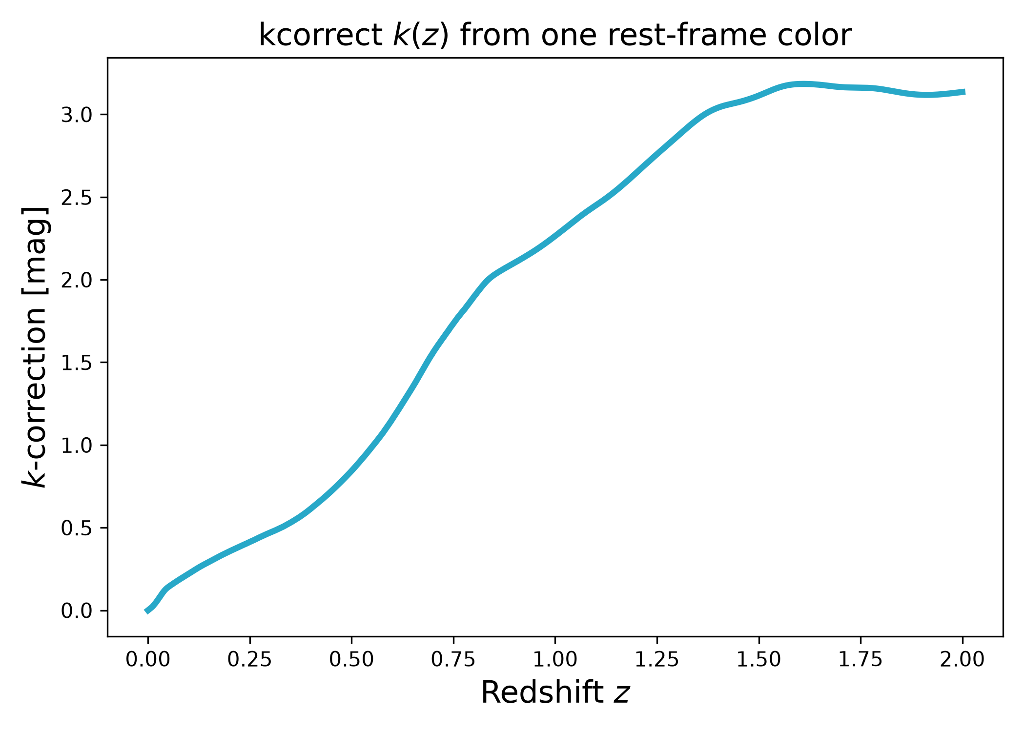
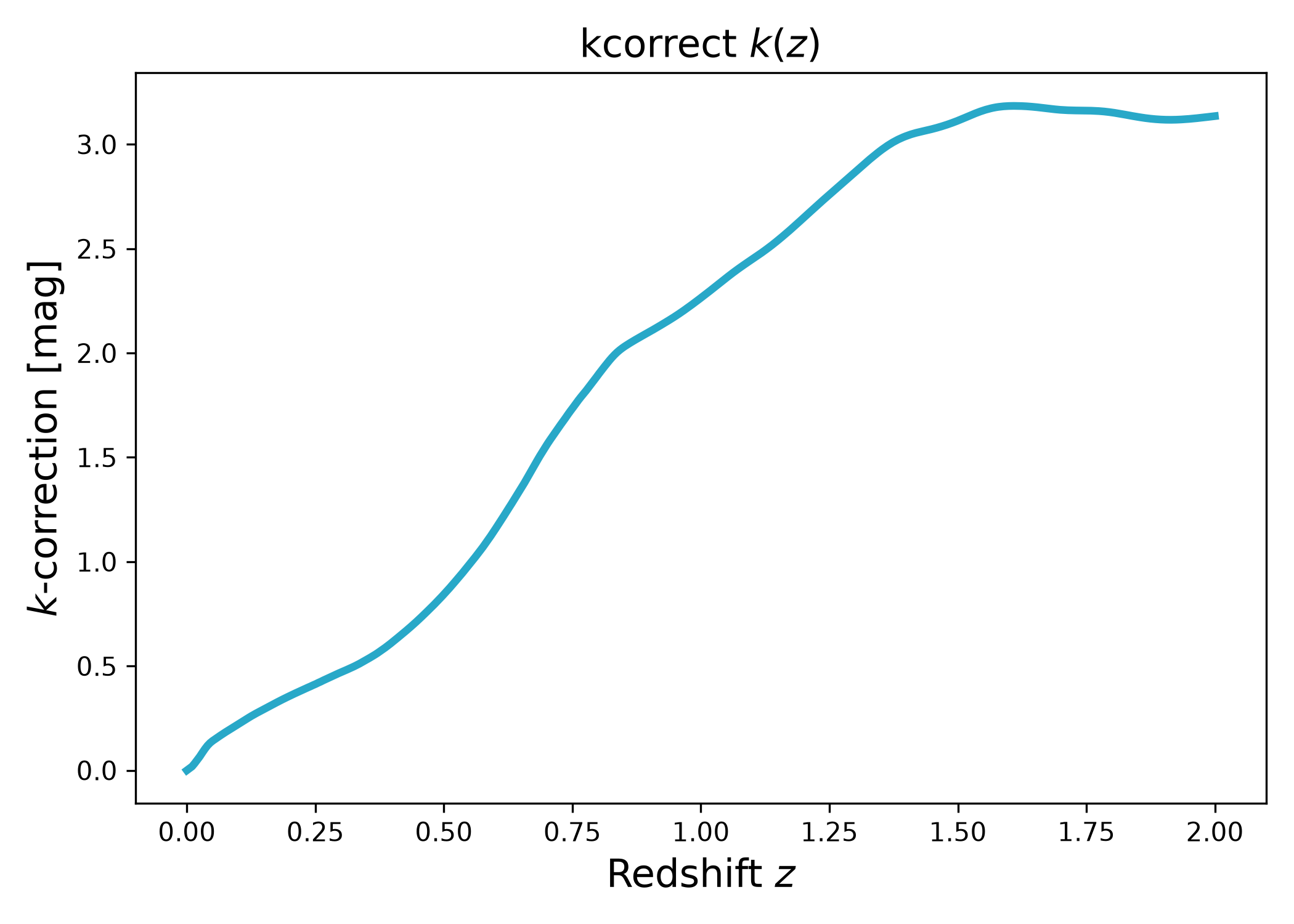
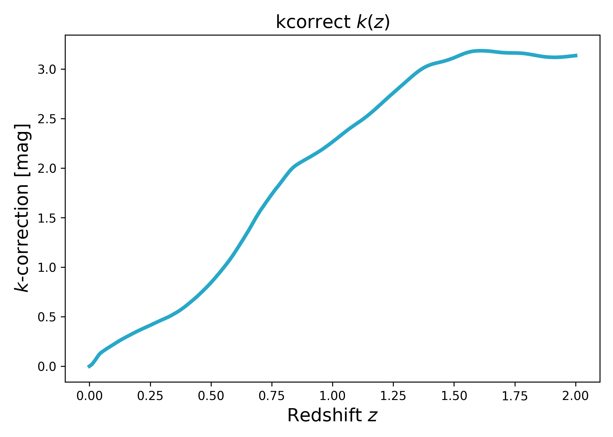
Basic kcorrect k(z) from a rest-frame color#
In this example we construct a lfkit.Corrections object from one
rest-frame color constraint and evaluate \(k(z)\) in a single output band.
import numpy as np
import matplotlib.pyplot as plt
import cmasher as cmr

from lfkit import Corrections

# Colors
cmap = "cmr.guppy"
c_red = cmr.take_cmap_colors(cmap, 3, cmap_range=(0.0, 0.2))[1]
c_blue = cmr.take_cmap_colors(cmap, 3, cmap_range=(0.8, 1.0))[1]

# Output response curve for which we want k(z)
response_out = "sdss_r0"

# One rest-frame color constraint: (band_a - band_b) at z_phot (default 0)
color = ("sdss_g0", "sdss_r0")
color_value = 0.8

corr = Corrections.kcorrect(
    response_out=response_out,
    color=color,
    color_value=color_value,
    anchor_z0=True,
)

z = np.linspace(0.0, 2.0, 500)
k = corr.k(z)

plt.figure(figsize=(7.0, 5.0))
plt.plot(z, k, lw=3, color=c_blue)
plt.xlabel("Redshift $z$", fontsize=15)
plt.ylabel("$k$-correction [mag]", fontsize=15)
plt.title("kcorrect $k(z)$ from one rest-frame color", fontsize=15)
plt.tight_layout()
(png)
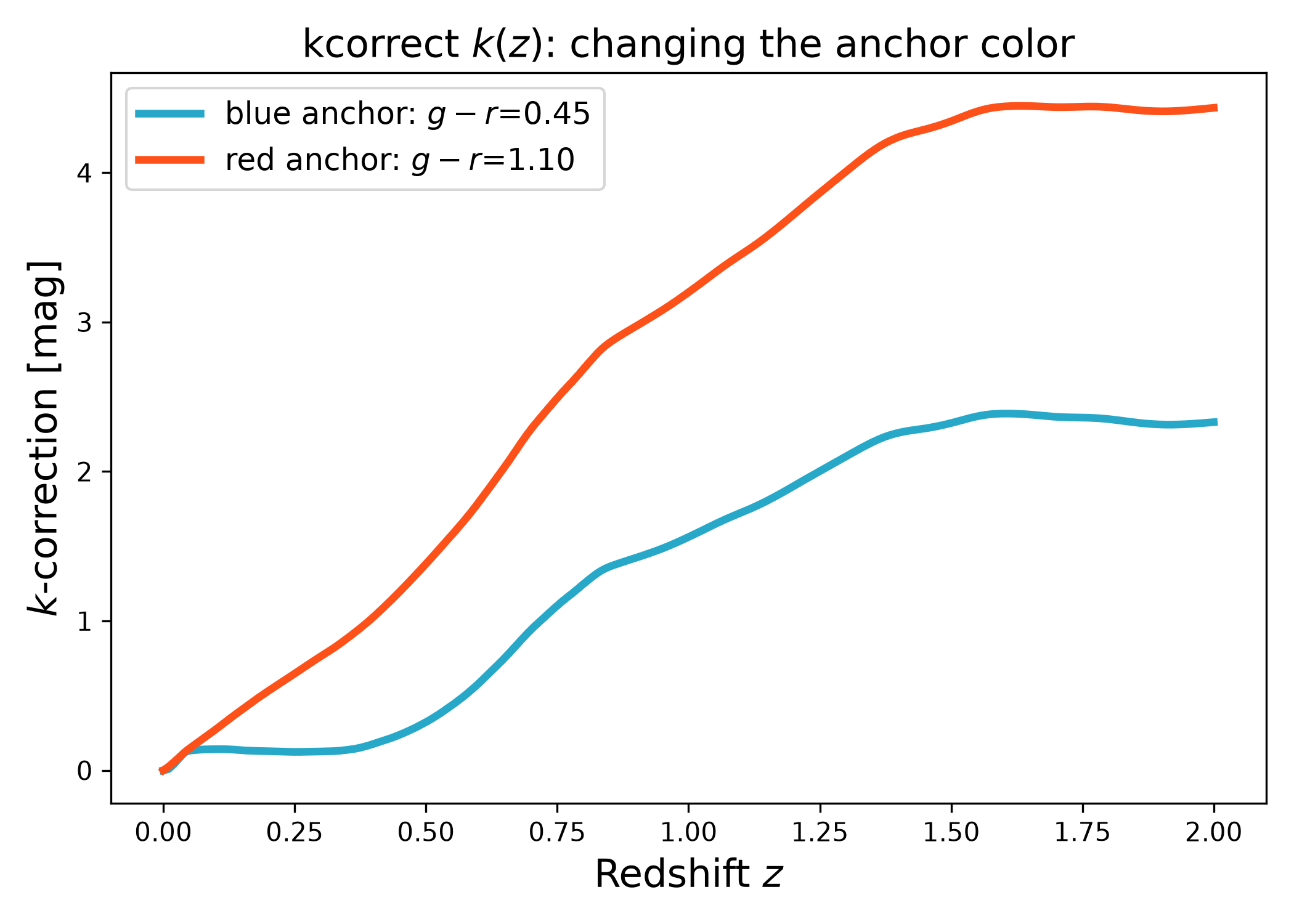
Red vs blue: vary the anchor color constraint#
Here we demonstrate “blue” vs “red” behavior by changing only the rest-frame color constraint (which changes the implied SED mixture).
import numpy as np
import matplotlib.pyplot as plt
import cmasher as cmr

from lfkit import Corrections

# Colors
cmap = "cmr.guppy"
c_red = cmr.take_cmap_colors(cmap, 3, cmap_range=(0.0, 0.2))[1]
c_blue = cmr.take_cmap_colors(cmap, 3, cmap_range=(0.8, 1.0))[1]

response_out = "sdss_r0"
color = ("sdss_g0", "sdss_r0")

# Two different rest-frame colors
color_blue = 0.45
color_red = 1.10

corr_blue = Corrections.kcorrect(
    response_out=response_out,
    color=color,
    color_value=color_blue,
    anchor_z0=True,
)

corr_red = Corrections.kcorrect(
    response_out=response_out,
    color=color,
    color_value=color_red,
    anchor_z0=True,
)

z = np.linspace(0.0, 2.0, 600)

plt.figure(figsize=(7.0, 5.0))
plt.plot(
    z, corr_blue.k(z), lw=3, color=c_blue,
    label=f"blue anchor: $g-r$={color_blue:.2f}"
)
plt.plot(
    z, corr_red.k(z), lw=3, color=c_red,
    label=f"red anchor: $g-r$={color_red:.2f}"
)
plt.xlabel("Redshift $z$", fontsize=15)
plt.ylabel("$k$-correction [mag]", fontsize=15)
plt.title("kcorrect $k(z)$: changing the anchor color", fontsize=15)
plt.legend(frameon=True, fontsize=12, loc="upper left")
plt.tight_layout()
(png)
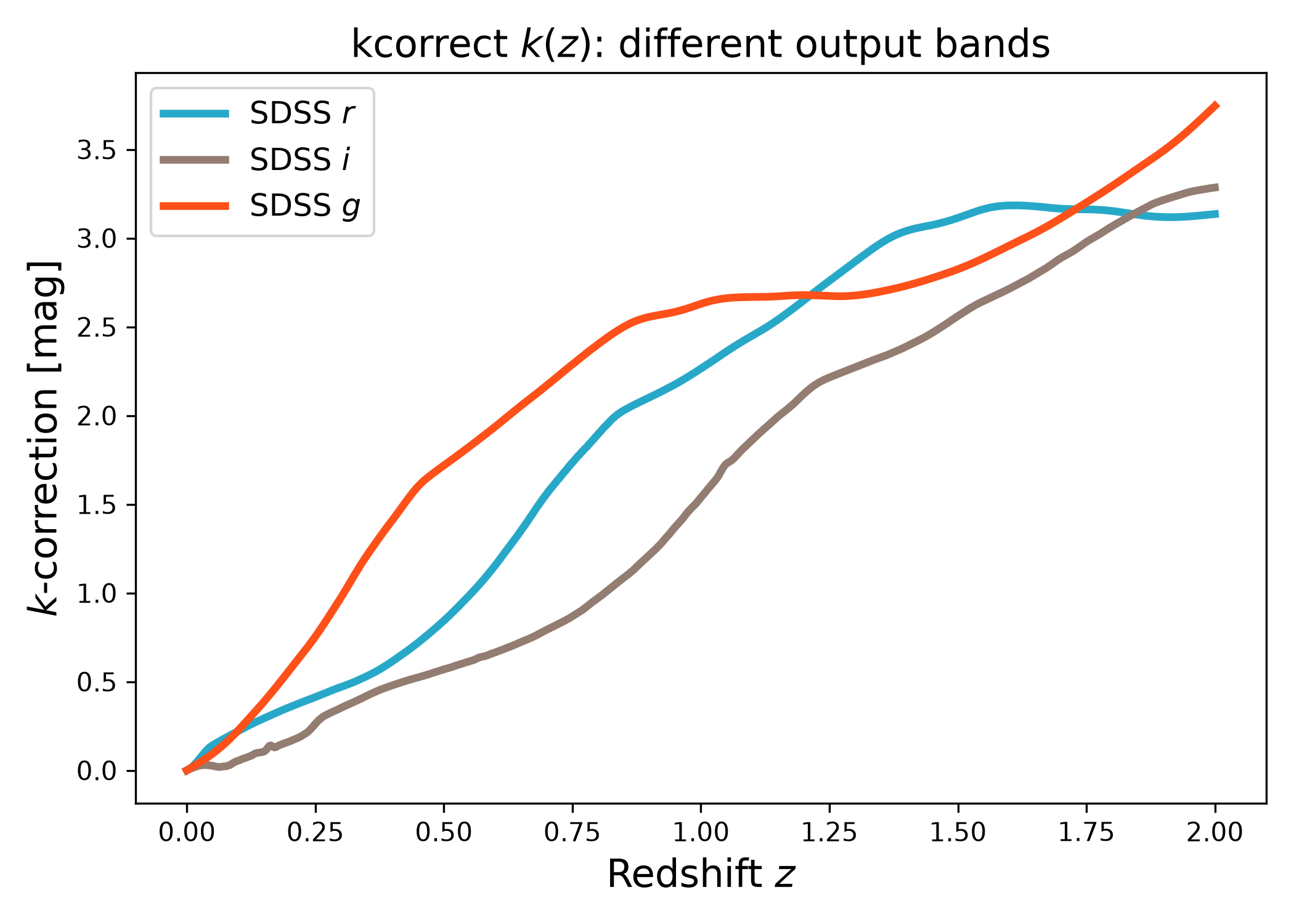
Output band choice: compute k(z) in different bands#
In this example we keep the same rest-frame color constraint, but evaluate \(k(z)\) in multiple output response bands.
import numpy as np
import matplotlib.pyplot as plt
import cmasher as cmr

from lfkit import Corrections

# Colors
cmap = "cmr.guppy"
c_red = cmr.take_cmap_colors(cmap, 3, cmap_range=(0.0, 0.2))[1]
c_blue = cmr.take_cmap_colors(cmap, 3, cmap_range=(0.8, 1.0))[1]

# One fixed rest-frame color constraint
color = ("sdss_g0", "sdss_r0")
color_value = 0.8

# Different output bands / responses
responses_out = [
    ("SDSS $r$", "sdss_r0"),
    ("SDSS $i$", "sdss_i0"),
    ("SDSS $g$", "sdss_g0"),
]

z = np.linspace(0.0, 2.0, 600)

plt.figure(figsize=(7.0, 5.0))

# Use a simple progression between the two anchor colors
colors = [c_blue, 0.5 * (np.array(c_blue) + np.array(c_red)), c_red]

for (label, response_out), c in zip(responses_out, colors):
    corr = Corrections.kcorrect(
        response_out=response_out,
        color=color,
        color_value=color_value,
        anchor_z0=True,
    )
    plt.plot(
        z, corr.k(z),
        lw=3,
        label=label, color=c)

plt.xlabel("Redshift $z$", fontsize=15)
plt.ylabel("$k$-correction [mag]", fontsize=15)
plt.title("kcorrect $k(z)$: different output bands", fontsize=15)
plt.legend(frameon=True, fontsize=12, loc="upper left")
plt.tight_layout()
(png)
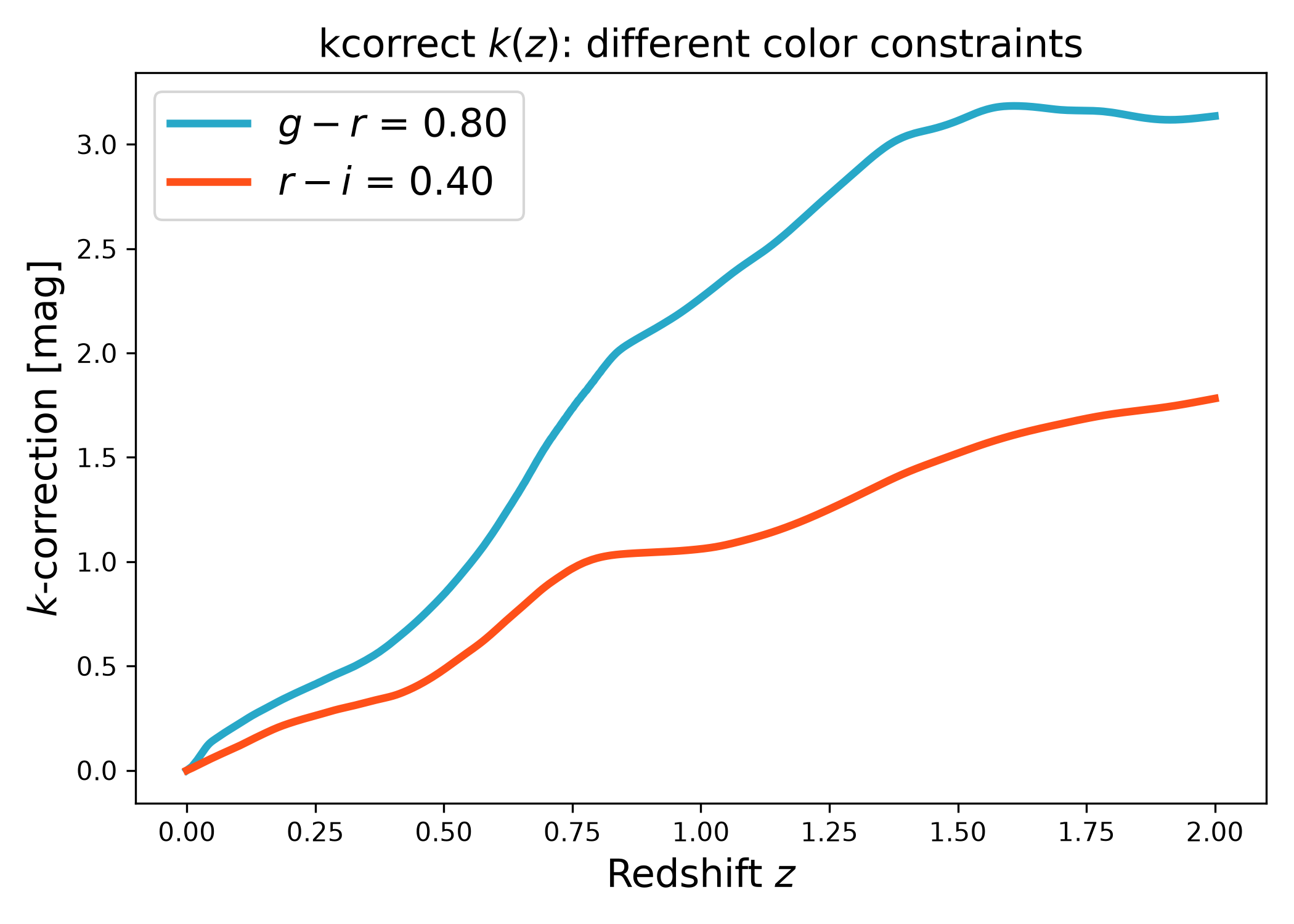
Different color definitions: (g-r) vs (r-i)#
Here we compare two commonly used rest-frame color definitions, \(g-r\) and \(r-i\), and show how each choice changes the inferred SED mixture and therefore \(k(z)\).
import numpy as np
import matplotlib.pyplot as plt
import cmasher as cmr

from lfkit import Corrections

# Colors
cmap = "cmr.guppy"
c_red = cmr.take_cmap_colors(cmap, 3, cmap_range=(0.0, 0.2))[1]
c_blue = cmr.take_cmap_colors(cmap, 3, cmap_range=(0.8, 1.0))[1]

response_out = "sdss_r0"

# Two commonly used rest-frame colors
color_gr = ("sdss_g0", "sdss_r0")
color_ri = ("sdss_r0", "sdss_i0")

color_gr_value = 0.80
color_ri_value = 0.40

corr_gr = Corrections.kcorrect(
    response_out=response_out,
    color=color_gr,
    color_value=color_gr_value,
    anchor_band="sdss_r0",
    anchor_z0=True,
)

corr_ri = Corrections.kcorrect(
    response_out=response_out,
    color=color_ri,
    color_value=color_ri_value,
    anchor_band="sdss_r0",
    anchor_z0=True,
)

z = np.linspace(0.0, 2.0, 600)

plt.figure(figsize=(7.0, 5.0))

plt.plot(
    z, corr_gr.k(z), lw=3, color=c_blue,
    label=f"$g-r$ = {color_gr_value:.2f}"
)

plt.plot(
    z, corr_ri.k(z), lw=3, color=c_red,
    label=f"$r-i$ = {color_ri_value:.2f}"
)

plt.xlabel("Redshift $z$", fontsize=15)
plt.ylabel("$k$-correction [mag]", fontsize=15)
plt.title("kcorrect $k(z)$: different color constraints", fontsize=15)
plt.legend(frameon=True, fontsize=15, loc="upper left")
plt.tight_layout()
(png)
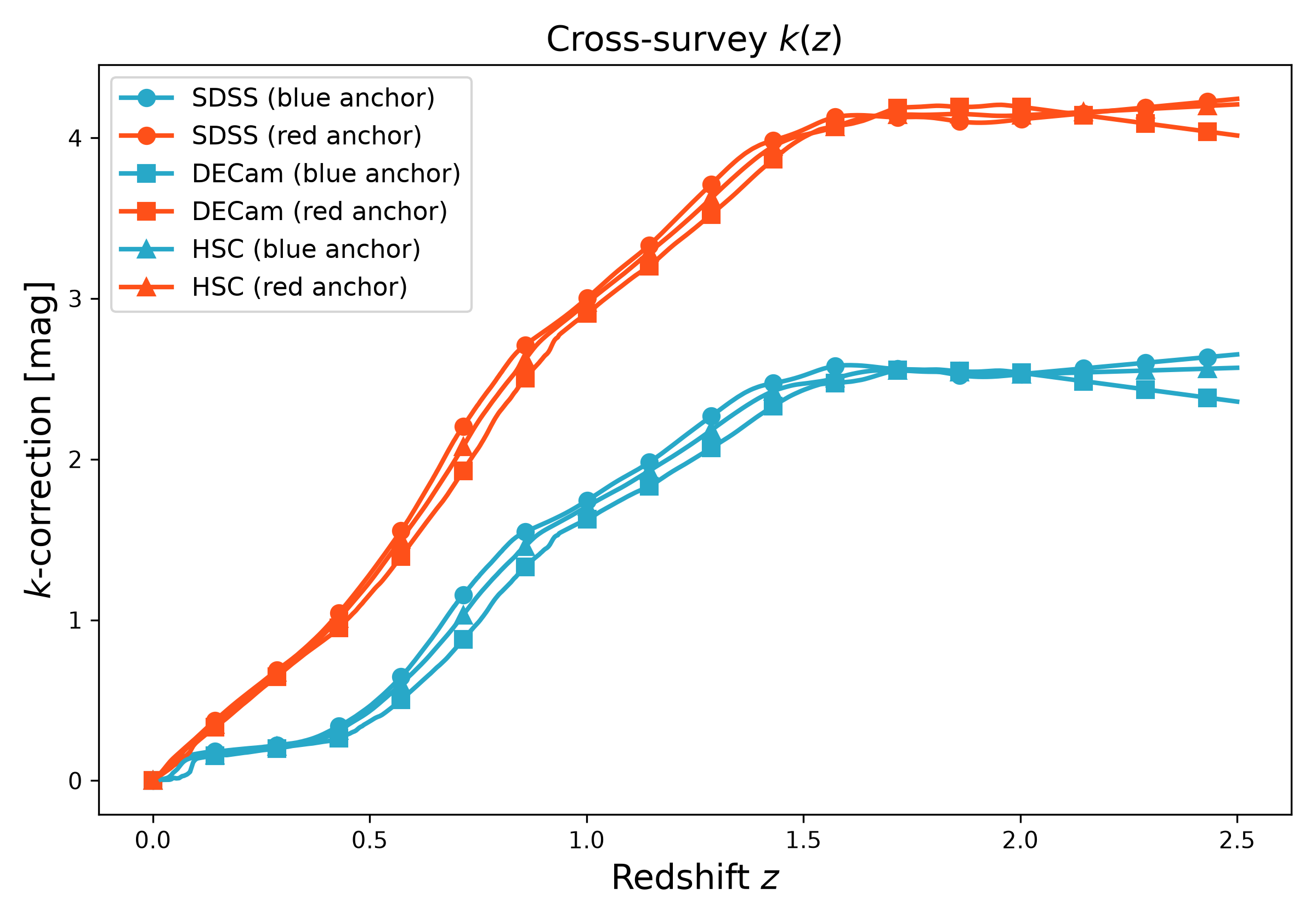
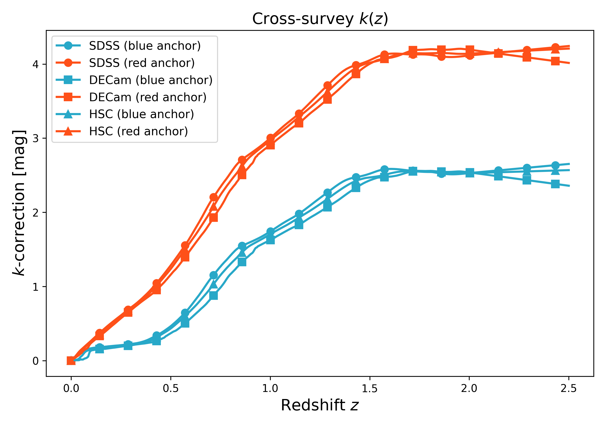
Cross-survey example: SDSS vs DECam vs HSC#
In this example we evaluate \(k(z)\) for multiple surveys (different output response curves) while keeping the same SDSS rest-frame color anchor.
If a response curve is missing in your local kcorrect installation, the example skips that survey so docs builds do not fail.
import numpy as np
import matplotlib.pyplot as plt
import cmasher as cmr

from lfkit import Corrections

# Colors
cmap = "cmr.guppy"
c_red = cmr.take_cmap_colors(cmap, 3, cmap_range=(0.0, 0.2))[1]
c_blue = cmr.take_cmap_colors(cmap, 3, cmap_range=(0.8, 1.0))[1]

# Keep the same rest-frame color anchor in SDSS responses
color = ("sdss_g0", "sdss_r0")
color_value_blue = 0.55
color_value_red = 1.05

surveys = [
    ("SDSS", "sdss_r0"),
    ("DECam", "decam_r"),
    ("HSC", "subaru_suprimecam_r"),
]

markers = {"SDSS": "o", "DECam": "s", "HSC": "^"}

z = np.linspace(0.0, 2.5, 700)

plt.figure(figsize=(8.0, 5.6))

for survey, response_out in surveys:
    try:
        corr_blue = Corrections.kcorrect(
            response_out=response_out,
            color=color,
            color_value=color_value_blue,
            anchor_z0=True,
        )
        corr_red = Corrections.kcorrect(
            response_out=response_out,
            color=color,
            color_value=color_value_red,
            anchor_z0=True,
        )
    except Exception:
        continue

    plt.plot(
        z, corr_blue.k(z),
        lw=2, marker=markers.get(survey, "o"), ms=7, markevery=40,
        color=c_blue,
        label=f"{survey} (blue anchor)"
    )
    plt.plot(
        z, corr_red.k(z),
        lw=2, marker=markers.get(survey, "s"), ms=7, markevery=40,
        color=c_red,
        label=f"{survey} (red anchor)"
    )

plt.xlabel("Redshift $z$", fontsize=15)
plt.ylabel("$k$-correction [mag]", fontsize=15)
plt.title("Cross-survey $k(z)$", fontsize=15)
plt.legend(frameon=True, fontsize=11, loc="upper left")
plt.tight_layout()
(png)
Listing available kcorrect responses#
This snippet lists response curve names available in your local kcorrect installation. LFKit can auto-discover the installed response directory.
from lfkit.corrections.responses import (
    discover_response_dir_auto,
    list_available_responses,
)

response_dir = discover_response_dir_auto()
print("kcorrect response_dir:", response_dir)

names = list_available_responses(response_dir)
print(f"Found {len(names)} responses. First 30:")
print(names[:30])
Inspecting metadata#
In this example we compute \(k(z)\) and also print a few entries from the
small meta dictionary stored on the lfkit.Corrections instance.
import numpy as np
import matplotlib.pyplot as plt
import cmasher as cmr

from lfkit import Corrections

# Colors
cmap = "cmr.guppy"
c_red = cmr.take_cmap_colors(cmap, 3, cmap_range=(0.0, 0.2))[1]
c_blue = cmr.take_cmap_colors(cmap, 3, cmap_range=(0.8, 1.0))[1]

corr = Corrections.kcorrect(
    response_out="sdss_r0",
    color=("sdss_g0", "sdss_r0"),
    color_value=0.8,
    anchor_z0=True,
)

# Plot k(z)
z = np.linspace(0.0, 2.0, 400)
plt.figure(figsize=(7.0, 5.0))
plt.plot(z, corr.k(z), lw=3, color=c_blue)
plt.xlabel("Redshift $z$", fontsize=15)
plt.ylabel("$k$-correction [mag]", fontsize=15)
plt.title("kcorrect $k(z)$", fontsize=15)
plt.tight_layout()

# Also print a few construction details to the build log
keys = [
    "k_backend",
    "response_out",
    "color",
    "color_value",
    "anchor_z0",
    "z_valid_min",
    "z_valid_max",
]
for k in keys:
    if k in corr.meta:
        print(f"{k}: {corr.meta[k]}")
(png)
Registering a custom response curve#
You can write a kcorrect-format .dat response curve file to a directory of
your choice, then point LFKit/kcorrect at that directory via response_dir=....
import numpy as np

from lfkit.corrections.responses import (
    write_kcorrect_response,
    list_available_responses,
    require_responses,
)

# Example toy response curve (replace with your real throughput data)
wave_A = np.linspace(3500.0, 9500.0, 400)  # Angstrom
thr = np.exp(-0.5 * ((wave_A - 6200.0) / 600.0) ** 2)

out_dir = "my_kcorrect_responses"
name = "my_survey_r"

write_kcorrect_response(
    name=name,
    wave_angst=wave_A,
    throughput=thr,
    out_dir=out_dir,
    normalize=True,
)

# Confirm it exists
print("Now available (first 30):", list_available_responses(out_dir)[:30])
require_responses([name], response_dir=out_dir)

# Use it as an output response in Corrections.kcorrect(...)
from lfkit import Corrections

corr = Corrections.kcorrect(
    response_out=name,
    color=("sdss_g0", "sdss_r0"),
    color_value=0.8,
    response_dir=out_dir,
    anchor_z0=True,
)