 LF-weighted redshift density#
This page shows how to convert a luminosity function into a redshift-dependent selection or weighting factor.
The redshift_density namespace is useful when constructing LF-dependent
redshift trends for survey forecasting. It combines an apparent magnitude limit
with a luminosity distance callable, integrates the luminosity function over the
visible absolute magnitude range, and can optionally apply a redshift or volume
weight.
This is not required to be a complete survey \(n(z)\) by itself. It is the LF-dependent ingredient that can be combined with survey geometry, volume weights, or tomography code.
All examples below are executable via .. plot::.
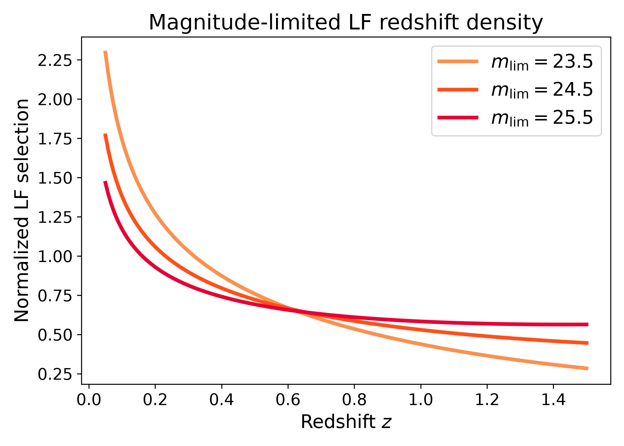
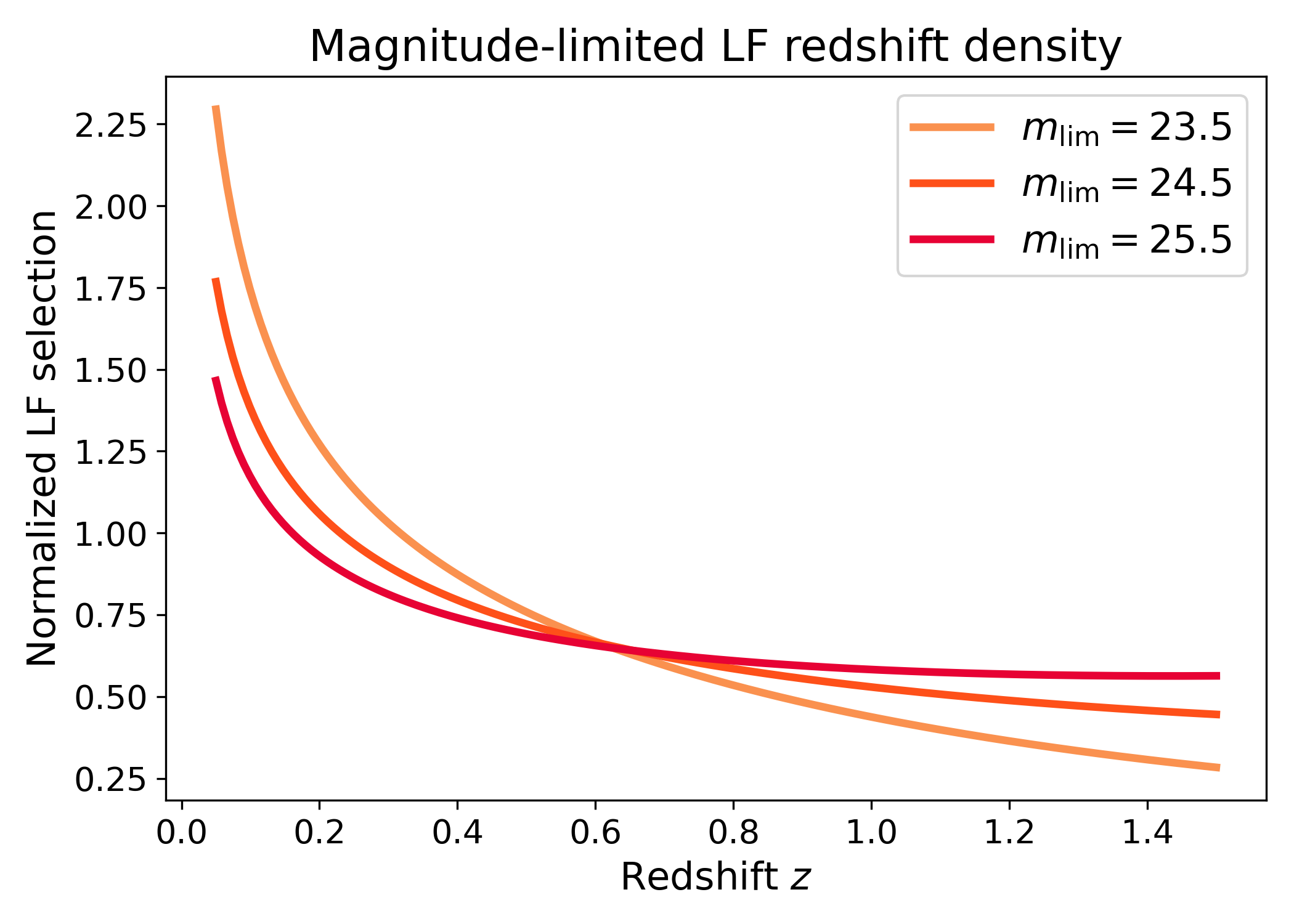
Magnitude-limited LF redshift density#
The integrated version computes the luminosity function number density selected by an apparent magnitude limit.
import numpy as np
import matplotlib.pyplot as plt
import cmasher as cmr

from lfkit import LuminosityFunction

LABEL_SIZE = 15
TICK_SIZE = 13
TITLE_SIZE = 17
LEGEND_SIZE = 15

lf = LuminosityFunction.evolving_schechter(
    phi_model="linear_p",
    phi_kwargs={"phi_0_star": 1.0e-3, "p": 0.7},
    m_star_model="linear_q",
    m_star_kwargs={"m_0_star": -20.5, "q": 0.8, "z_ref": 0.1},
    alpha_model="constant",
    alpha_kwargs={"alpha": -1.1},
)

redshift = np.linspace(0.05, 1.5, 180)

def luminosity_distance_mpc(z):
    return 3000.0 * z * (1.0 + 0.5 * z)

limits = [23.5, 24.5, 25.5]
colors = cmr.take_cmap_colors("cmr.guppy", len(limits), cmap_range=(0.0, 0.2))

fig, ax = plt.subplots(figsize=(7.0, 5.0))

for m_lim, color in zip(limits, colors):
    number_density = lf.redshift_density.integrated_number_density(
        redshift,
        m_lim=m_lim,
        m_bright=-24.0,
        luminosity_distance_mpc_fn=luminosity_distance_mpc,
        n_m=800,
    )

    number_density /= np.trapezoid(number_density, redshift)

    ax.plot(
        redshift,
        number_density,
        lw=3,
        color=color,
        label=rf"$m_{{\rm lim}}={m_lim}$",
    )

ax.set_xlabel("Redshift $z$", fontsize=LABEL_SIZE)
ax.set_ylabel("Normalized LF selection", fontsize=LABEL_SIZE)
ax.set_title("Magnitude-limited LF redshift density", fontsize=TITLE_SIZE)
ax.tick_params(axis="both", labelsize=TICK_SIZE)
ax.legend(frameon=True, fontsize=LEGEND_SIZE, loc="best")
plt.tight_layout()
(png)
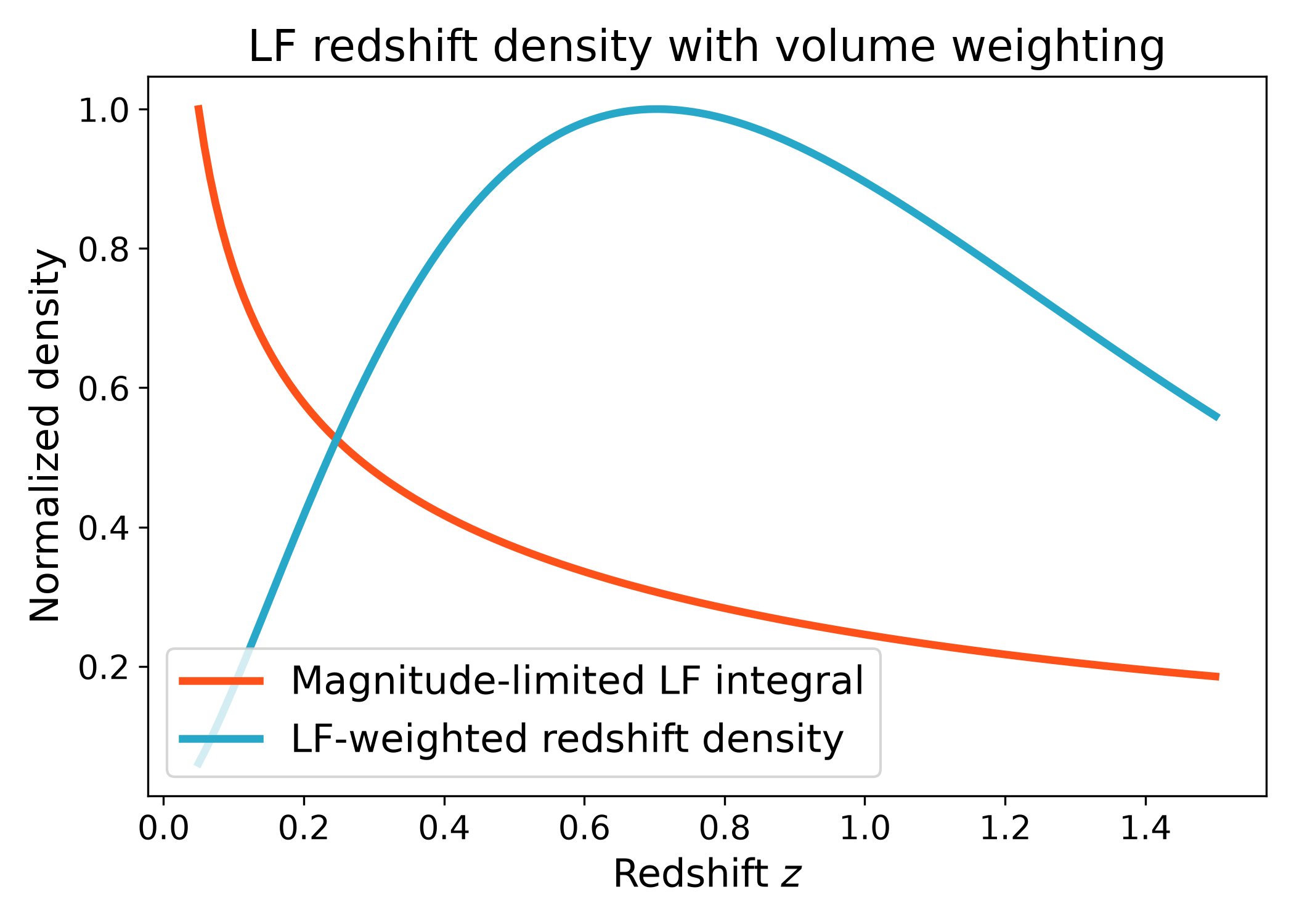
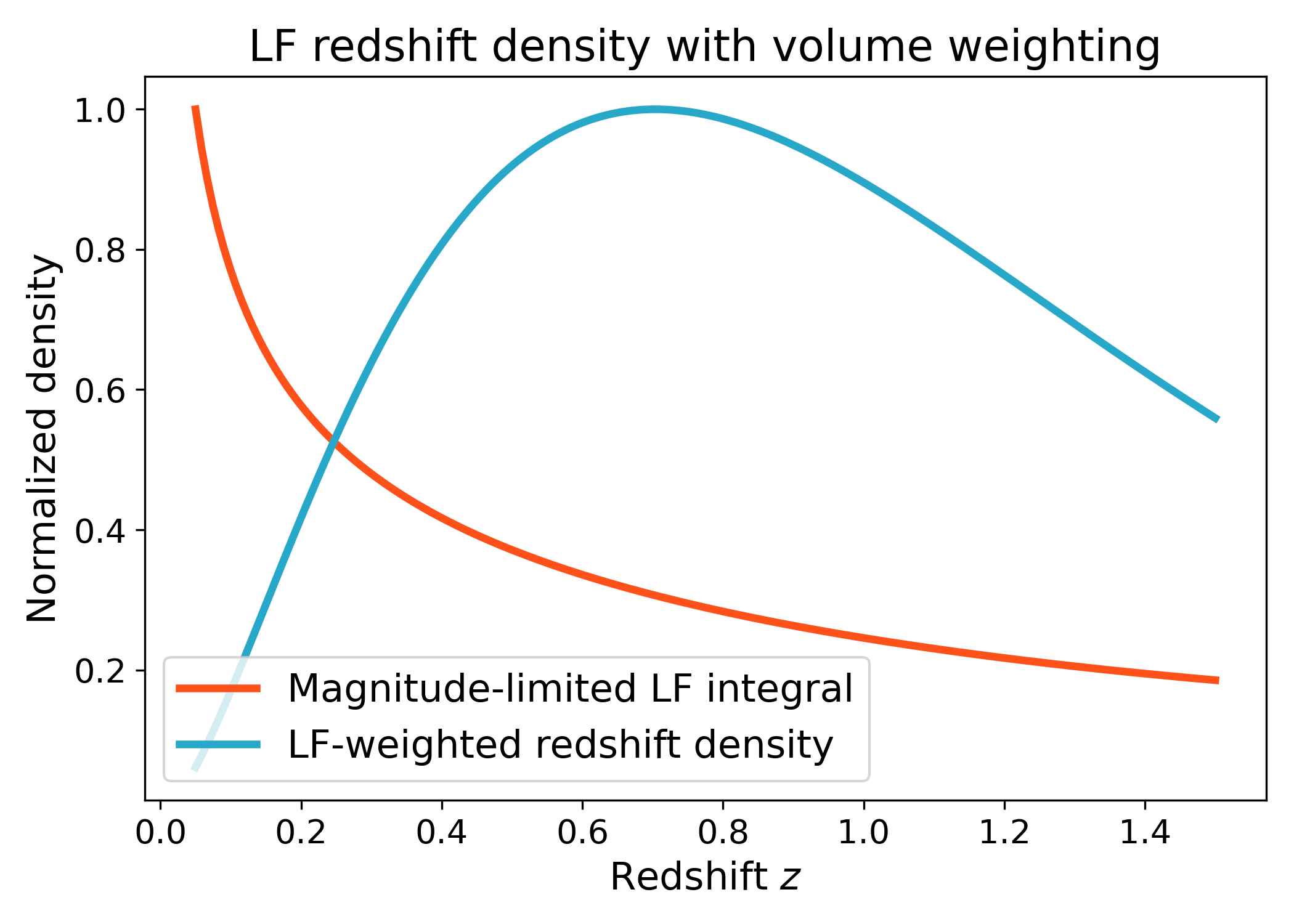
LF-weighted redshift trend#
The weighted version multiplies the magnitude-integrated luminosity function by a user-provided redshift or volume weight.
import numpy as np
import matplotlib.pyplot as plt
import cmasher as cmr

from lfkit import LuminosityFunction

LABEL_SIZE = 15
TICK_SIZE = 13
TITLE_SIZE = 17
LEGEND_SIZE = 15

lf = LuminosityFunction.evolving_schechter(
    phi_model="linear_p",
    phi_kwargs={"phi_0_star": 1.0e-3, "p": 0.7},
    m_star_model="linear_q",
    m_star_kwargs={"m_0_star": -20.5, "q": 0.8, "z_ref": 0.1},
    alpha_model="constant",
    alpha_kwargs={"alpha": -1.1},
)

redshift = np.linspace(0.05, 1.5, 180)

def luminosity_distance_mpc(z):
    return 3000.0 * z * (1.0 + 0.5 * z)

def volume_weight(z):
    return z**2 * np.exp(-z / 0.5)

number_density = lf.redshift_density.integrated_number_density(
    redshift,
    m_lim=24.0,
    m_bright=-24.0,
    luminosity_distance_mpc_fn=luminosity_distance_mpc,
    n_m=800,
)

weighted_density = lf.redshift_density.weighted(
    redshift,
    m_lim=24.0,
    m_bright=-24.0,
    luminosity_distance_mpc_fn=luminosity_distance_mpc,
    volume_weight_fn=volume_weight,
    n_m=800,
)

red = cmr.take_cmap_colors("cmr.guppy", 3, cmap_range=(0.0, 0.2))[1]
blue = cmr.take_cmap_colors("cmr.guppy", 3, cmap_range=(0.8, 1.0))[1]

fig, ax = plt.subplots(figsize=(7.0, 5.0))
ax.plot(
    redshift,
    number_density / np.max(number_density),
    lw=3,
    color=red,
    label="Magnitude-limited LF integral",
)
ax.plot(
    redshift,
    weighted_density / np.max(weighted_density),
    lw=3,
    color=blue,
    label="LF-weighted redshift density",
)

ax.set_xlabel("Redshift $z$", fontsize=LABEL_SIZE)
ax.set_ylabel("Normalized density", fontsize=LABEL_SIZE)
ax.set_title("LF redshift density with volume weighting", fontsize=TITLE_SIZE)
ax.tick_params(axis="both", labelsize=TICK_SIZE)
ax.legend(frameon=True, fontsize=LEGEND_SIZE, loc="best")
plt.tight_layout()
(png)
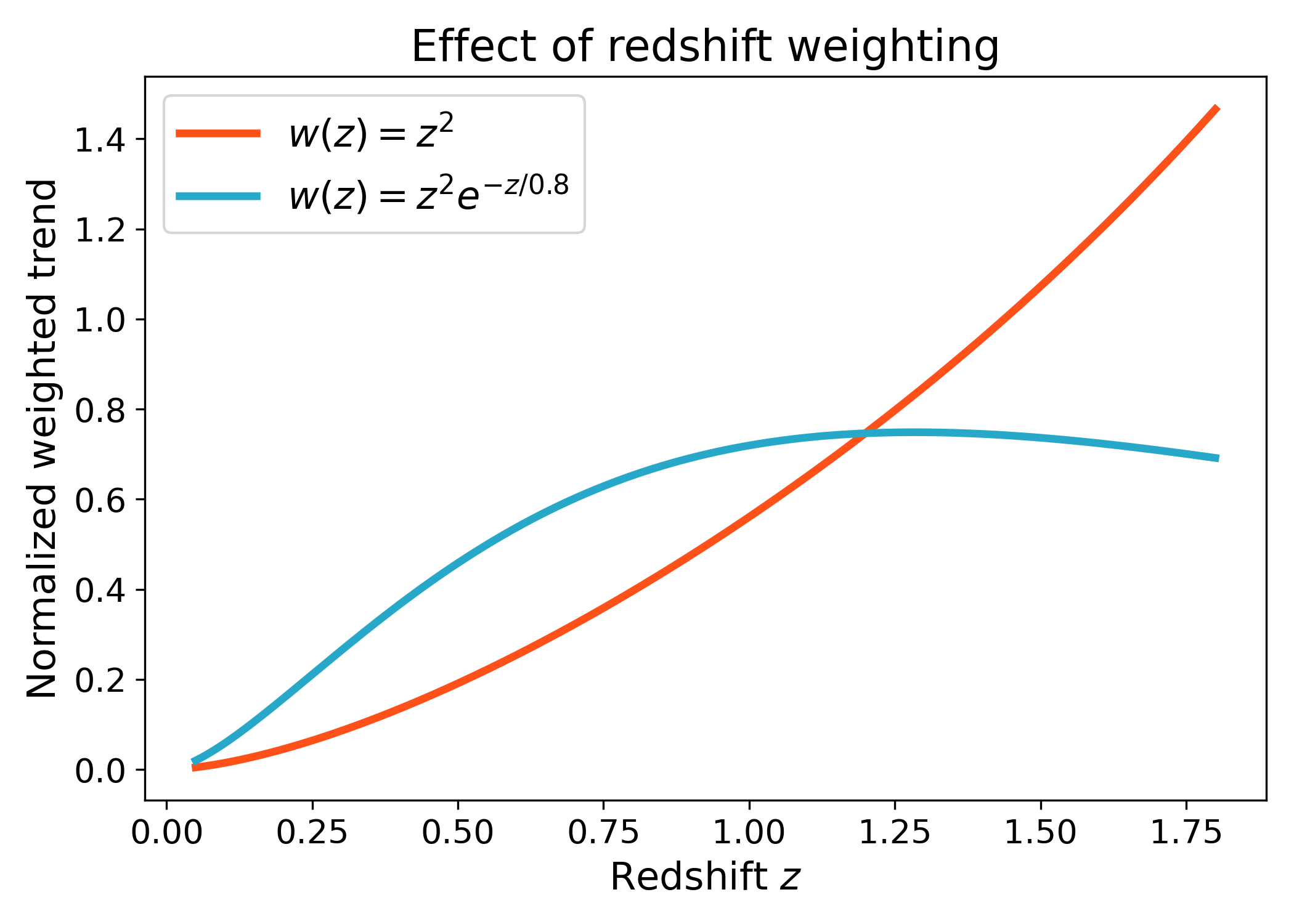
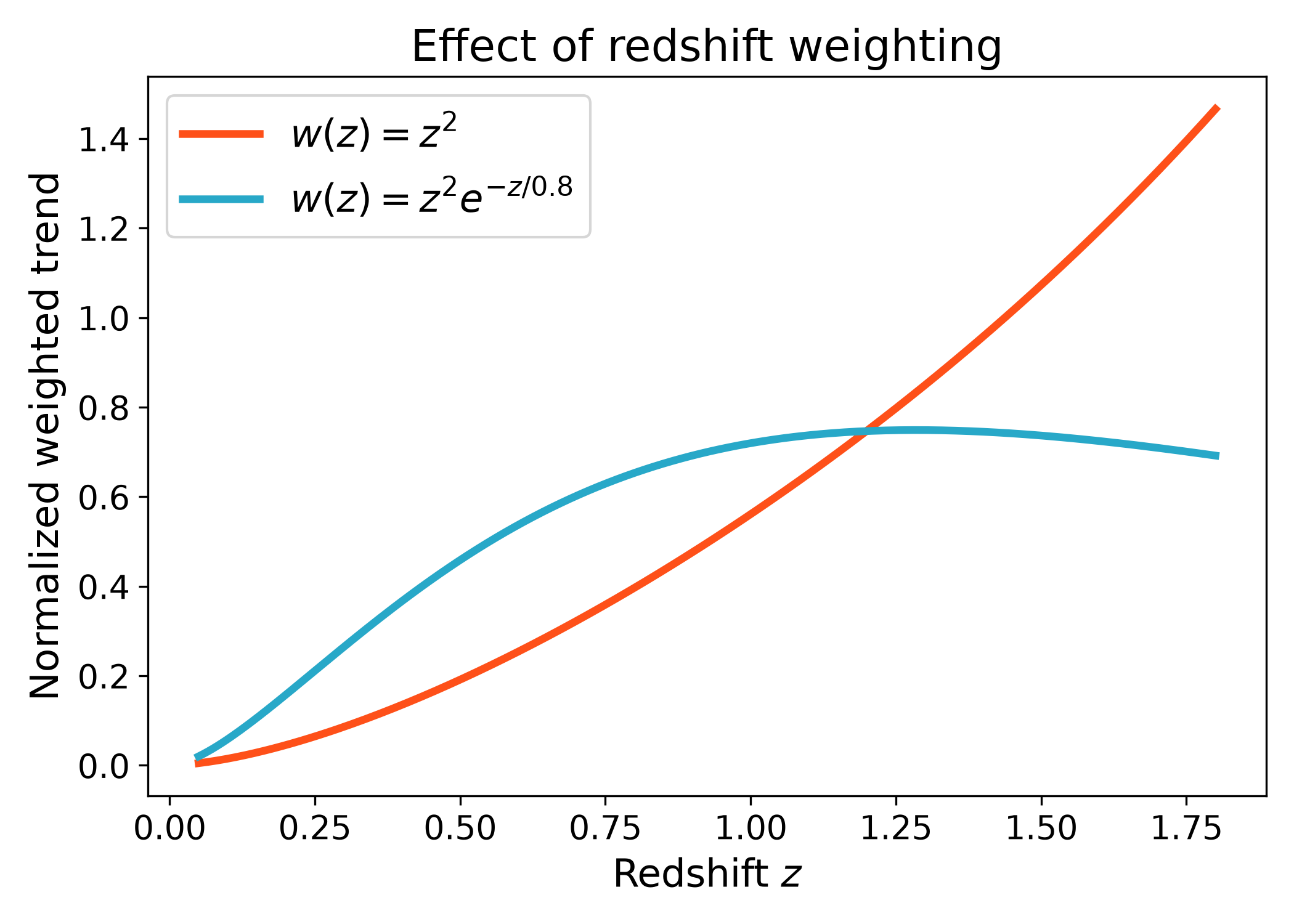
Cosmology-style volume weighting#
A common survey ingredient is a volume-like weight. The example below uses a simple callable to keep the redshift-density API independent of any specific cosmology backend.
import numpy as np
import matplotlib.pyplot as plt
import cmasher as cmr

from lfkit import LuminosityFunction

LABEL_SIZE = 15
TICK_SIZE = 13
TITLE_SIZE = 17
LEGEND_SIZE = 15

lf = LuminosityFunction.evolving_schechter(
    phi_model="linear_p",
    phi_kwargs={"phi_0_star": 1.0e-3, "p": 0.6},
    m_star_model="linear_q",
    m_star_kwargs={"m_0_star": -20.5, "q": 0.8, "z_ref": 0.1},
    alpha_model="constant",
    alpha_kwargs={"alpha": -1.1},
)

redshift = np.linspace(0.05, 1.8, 220)

def luminosity_distance_mpc(z):
    return 3000.0 * z * (1.0 + 0.4 * z)

def low_z_volume_weight(z):
    return z**2

def tapered_volume_weight(z):
    return z**2 * np.exp(-z / 0.8)

low_z_trend = lf.redshift_density.weighted(
    redshift,
    m_lim=24.5,
    m_bright=-24.0,
    luminosity_distance_mpc_fn=luminosity_distance_mpc,
    volume_weight_fn=low_z_volume_weight,
    n_m=800,
)

tapered_trend = lf.redshift_density.weighted(
    redshift,
    m_lim=24.5,
    m_bright=-24.0,
    luminosity_distance_mpc_fn=luminosity_distance_mpc,
    volume_weight_fn=tapered_volume_weight,
    n_m=800,
)

low_z_trend /= np.trapezoid(low_z_trend, redshift)
tapered_trend /= np.trapezoid(tapered_trend, redshift)

red = cmr.take_cmap_colors("cmr.guppy", 3, cmap_range=(0.0, 0.2))[1]
blue = cmr.take_cmap_colors("cmr.guppy", 3, cmap_range=(0.8, 1.0))[1]

fig, ax = plt.subplots(figsize=(7.0, 5.0))
ax.plot(redshift, low_z_trend, lw=3, color=red, label=r"$w(z)=z^2$")
ax.plot(redshift, tapered_trend, lw=3, color=blue, label=r"$w(z)=z^2 e^{-z/0.8}$")

ax.set_xlabel("Redshift $z$", fontsize=LABEL_SIZE)
ax.set_ylabel("Normalized weighted trend", fontsize=LABEL_SIZE)
ax.set_title("Effect of redshift weighting", fontsize=TITLE_SIZE)
ax.tick_params(axis="both", labelsize=TICK_SIZE)
ax.legend(frameon=True, fontsize=LEGEND_SIZE, loc="best")
plt.tight_layout()
(png)