 Luminosity function fractions#
This page shows how to compute population fractions from luminosity functions.
The fractions namespace is useful when one luminosity function describes a
subsample and another luminosity function describes the full sample. For example,
the numerator could be a red galaxy luminosity function and the denominator could
be the total galaxy luminosity function. The resulting fraction is an integrated
quantity: both luminosity functions are integrated over the same absolute
magnitude range, and the ratio of those integrals is returned.
This is useful for comparing how the relative abundance of a population changes with redshift, magnitude selection, sample depth, or model choice.
In the examples below, we often use red and blue luminosity functions as
a simple cosmology motivated population split. In this context, red samples are
often used as a rough proxy for elliptical or early type galaxies, while blue
samples are often used as a rough proxy for spiral or late type galaxies. This
is a simplified classification, but it is common in galaxy evolution and
cosmology applications.
The same functions can be used for any pair of galaxy populations, not only red and blue samples. For example, the numerator could describe star forming galaxies, quenched galaxies, centrals, satellites, emission line galaxies, or any other selected subsample. In each case, the denominator should describe the full population relative to which the fraction is meant to be interpreted.
The denominator can be another LuminosityFunction instance or a callable. A
callable denominator should accept absolute magnitude and redshift as positional
arguments:
def denominator_lf(absolute_mag, redshift):
    return phi_total
All examples below are executable via .. plot::.
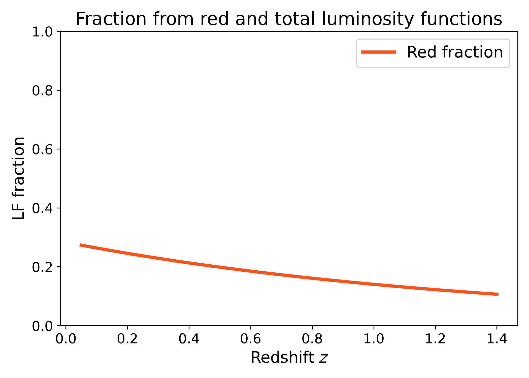
Red fraction from two luminosity functions#
The most direct use is to bind the numerator luminosity function and pass the
denominator luminosity function to fraction.
In this example, the numerator is a red galaxy luminosity function and the denominator is a total galaxy luminosity function. The plotted curve shows how the integrated red fraction evolves with redshift for a fixed absolute magnitude range. This is the typical use case when the sample selection is fixed and one wants to study population evolution.
import numpy as np
import matplotlib.pyplot as plt
import cmasher as cmr

from lfkit import LuminosityFunction

LABEL_SIZE = 15
TICK_SIZE = 13
TITLE_SIZE = 17
LEGEND_SIZE = 15

red_lf = LuminosityFunction.evolving_schechter(
    phi_model="linear_p",
    phi_kwargs={"phi_0_star": 5.0e-4, "p": -0.2},
    m_star_model="linear_q",
    m_star_kwargs={"m_0_star": -20.4, "q": 0.5, "z_ref": 0.1},
    alpha_model="constant",
    alpha_kwargs={"alpha": -0.8},
)

all_lf = LuminosityFunction.evolving_schechter(
    phi_model="linear_p",
    phi_kwargs={"phi_0_star": 1.2e-3, "p": 0.4},
    m_star_model="linear_q",
    m_star_kwargs={"m_0_star": -20.6, "q": 0.7, "z_ref": 0.1},
    alpha_model="constant",
    alpha_kwargs={"alpha": -1.1},
)

redshift = np.linspace(0.05, 1.4, 120)

red_fraction = np.array(
    [
        red_lf.fractions.fraction(
            z,
            all_lf,
            m_bright=-24.0,
            m_faint=-18.0,
            n_m=600,
        )
        for z in redshift
    ]
)

red = cmr.take_cmap_colors("cmr.guppy", 3, cmap_range=(0.0, 0.2))[1]

fig, ax = plt.subplots(figsize=(7.0, 5.0))
ax.plot(
    redshift,
    red_fraction,
    lw=3,
    color=red,
    label="Red fraction",
)

ax.set_xlabel("Redshift $z$", fontsize=LABEL_SIZE)
ax.set_ylabel("LF fraction", fontsize=LABEL_SIZE)
ax.set_title("Fraction from red and total luminosity functions", fontsize=TITLE_SIZE)
ax.tick_params(axis="both", labelsize=TICK_SIZE)
ax.set_ylim(0.0, 1.0)
ax.legend(frameon=True, fontsize=LEGEND_SIZE, loc="best")
plt.tight_layout()
(png)
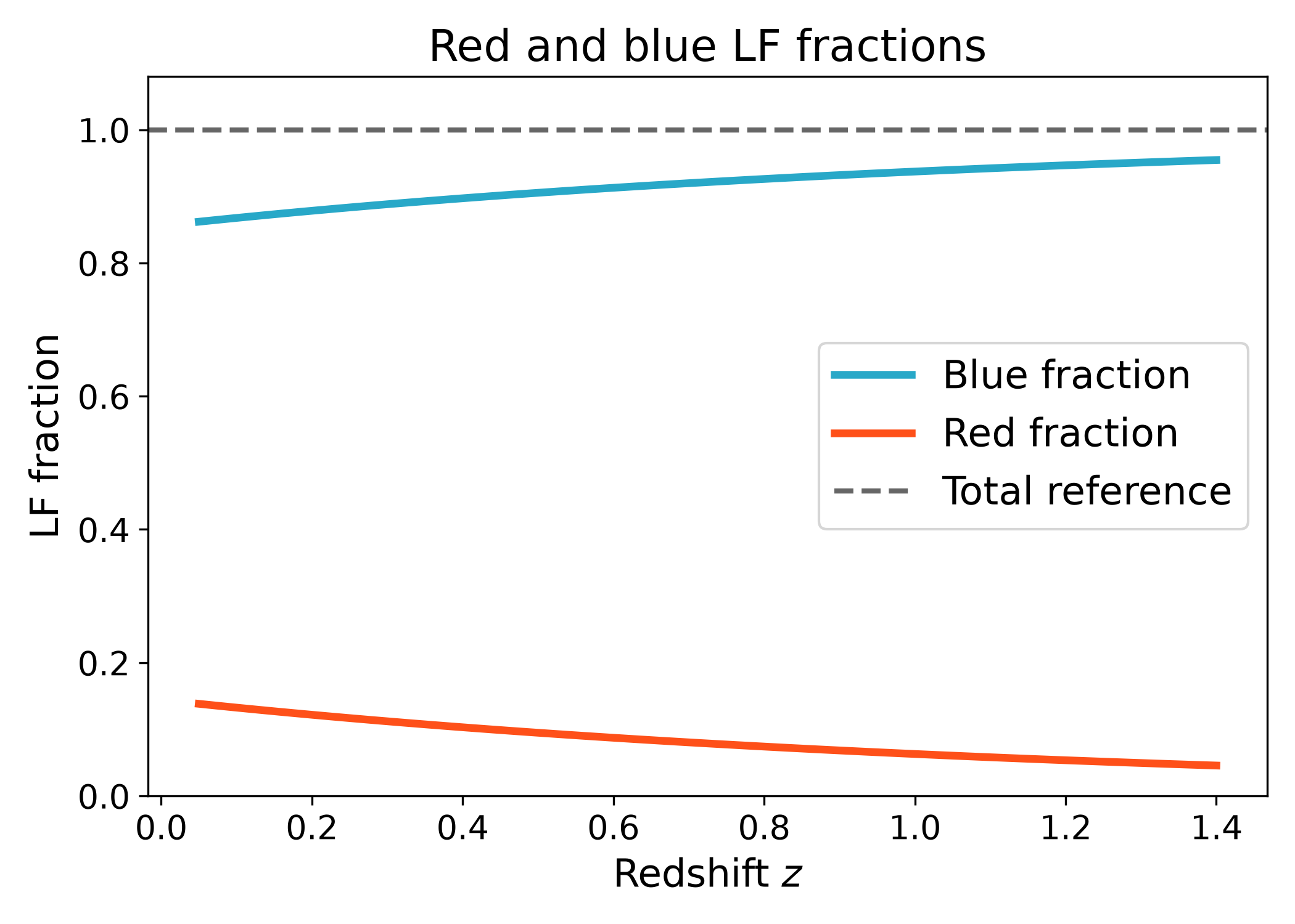
Red and blue fractions#
The red_fraction and blue_fraction helpers are convenience methods for
the common color split case. The blue fraction is the complement of the red
fraction with respect to the denominator luminosity function. The total fraction
is shown as a reference line at one.
This plot is a useful sanity check for two population fractions. If the red
fraction increases, the blue fraction decreases by the same amount because the
blue fraction is defined as 1 - red_fraction. This is appropriate when the
denominator represents the full sample and the numerator represents one
subsample.
import numpy as np
import matplotlib.pyplot as plt
import cmasher as cmr

from lfkit import LuminosityFunction

LABEL_SIZE = 15
TICK_SIZE = 13
TITLE_SIZE = 17
LEGEND_SIZE = 15

red_lf = LuminosityFunction.evolving_schechter(
    phi_model="linear_p",
    phi_kwargs={"phi_0_star": 3.5e-4, "p": -0.4},
    m_star_model="linear_q",
    m_star_kwargs={"m_0_star": -20.3, "q": 0.4, "z_ref": 0.1},
    alpha_model="constant",
    alpha_kwargs={"alpha": -0.7},
)

all_lf = LuminosityFunction.evolving_schechter(
    phi_model="linear_p",
    phi_kwargs={"phi_0_star": 1.4e-3, "p": 0.3},
    m_star_model="linear_q",
    m_star_kwargs={"m_0_star": -20.7, "q": 0.7, "z_ref": 0.1},
    alpha_model="constant",
    alpha_kwargs={"alpha": -1.1},
)

redshift = np.linspace(0.05, 1.4, 120)

red_fraction = np.array(
    [
        red_lf.fractions.red_fraction(
            z,
            all_lf,
            m_bright=-24.0,
            m_faint=-18.0,
            n_m=600,
        )
        for z in redshift
    ]
)

blue_fraction = np.array(
    [
        red_lf.fractions.blue_fraction(
            z,
            all_lf,
            m_bright=-24.0,
            m_faint=-18.0,
            n_m=600,
        )
        for z in redshift
    ]
)

red = cmr.take_cmap_colors("cmr.guppy", 3, cmap_range=(0.0, 0.2))[1]
blue = cmr.take_cmap_colors("cmr.guppy", 3, cmap_range=(0.8, 1.0))[1]

fig, ax = plt.subplots(figsize=(7.0, 5.0))
ax.plot(
    redshift,
    blue_fraction,
    lw=3,
    color=blue,
    label="Blue fraction",
)
ax.plot(
    redshift,
    red_fraction,
    lw=3,
    color=red,
    label="Red fraction",
)
ax.axhline(
    1.0,
    color="k",
    lw=2,
    ls="--",
    alpha=0.6,
    label="Total reference",
)

ax.set_xlabel("Redshift $z$", fontsize=LABEL_SIZE)
ax.set_ylabel("LF fraction", fontsize=LABEL_SIZE)
ax.set_title("Red and blue LF fractions", fontsize=TITLE_SIZE)
ax.tick_params(axis="both", labelsize=TICK_SIZE)
ax.set_ylim(0.0, 1.08)
ax.legend(frameon=True, fontsize=LEGEND_SIZE, loc="best")
plt.tight_layout()
(png)

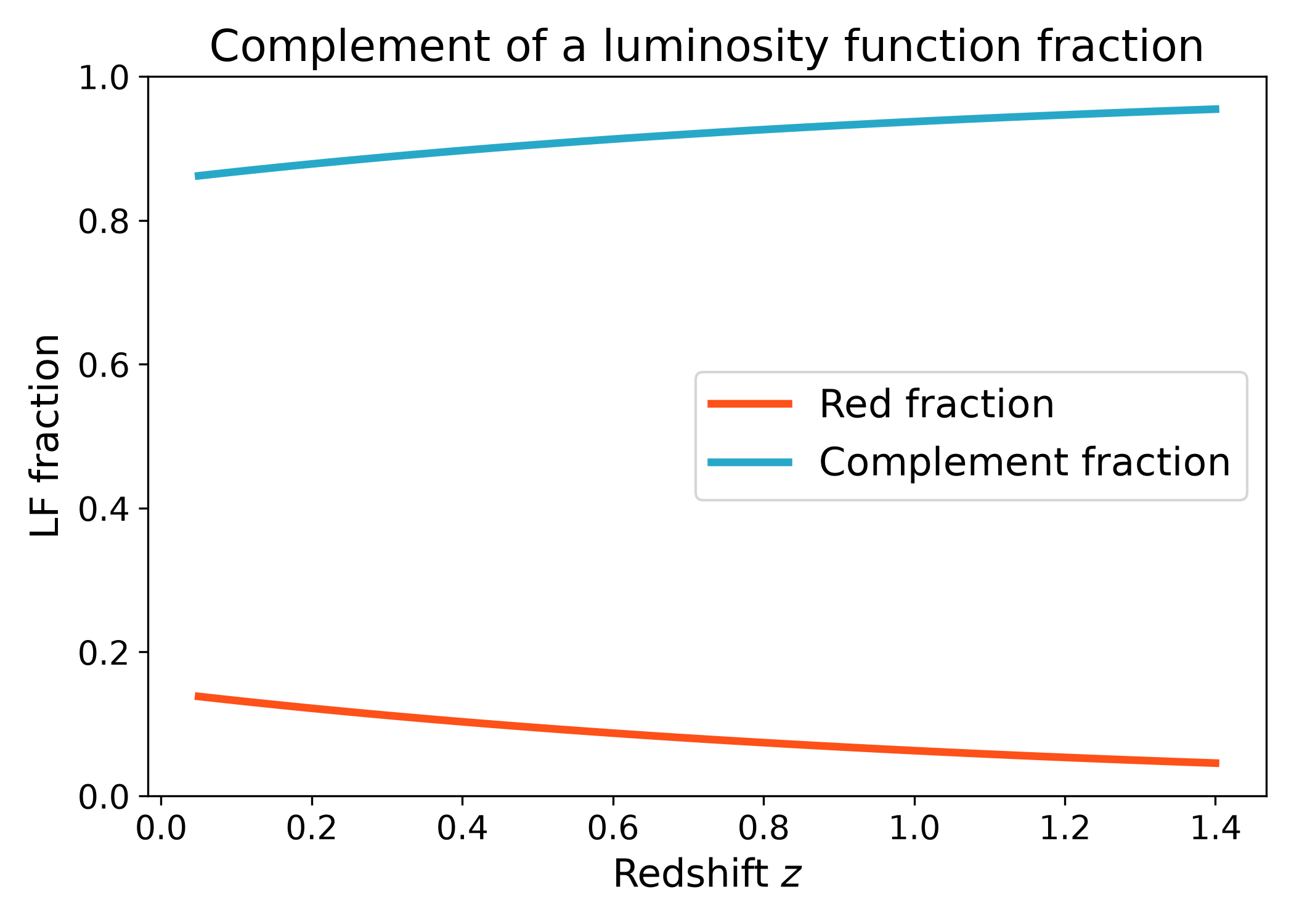
Complement fraction#
Sometimes one luminosity function describes a selected population and another describes the full population. In that case the complement fraction is useful for the population not described by the numerator. For example, if the numerator is the red luminosity function, then the complement is the blue fraction with respect to the total luminosity function.
This is useful when only one subsample luminosity function is available. Instead of explicitly modeling the second subsample, the complement gives the remaining fraction implied by the chosen numerator and denominator models.
import numpy as np
import matplotlib.pyplot as plt
import cmasher as cmr

from lfkit import LuminosityFunction

LABEL_SIZE = 15
TICK_SIZE = 13
TITLE_SIZE = 17
LEGEND_SIZE = 15

red_lf = LuminosityFunction.evolving_schechter(
    phi_model="linear_p",
    phi_kwargs={"phi_0_star": 3.5e-4, "p": -0.4},
    m_star_model="linear_q",
    m_star_kwargs={"m_0_star": -20.3, "q": 0.4, "z_ref": 0.1},
    alpha_model="constant",
    alpha_kwargs={"alpha": -0.7},
)

all_lf = LuminosityFunction.evolving_schechter(
    phi_model="linear_p",
    phi_kwargs={"phi_0_star": 1.4e-3, "p": 0.3},
    m_star_model="linear_q",
    m_star_kwargs={"m_0_star": -20.7, "q": 0.7, "z_ref": 0.1},
    alpha_model="constant",
    alpha_kwargs={"alpha": -1.1},
)

redshift = np.linspace(0.05, 1.4, 120)

red_fraction = np.array(
    [
        red_lf.fractions.red_fraction(
            z,
            all_lf,
            m_bright=-24.0,
            m_faint=-18.0,
            n_m=600,
        )
        for z in redshift
    ]
)

complement_fraction = np.array(
    [
        red_lf.fractions.complement_fraction(
            z,
            all_lf,
            m_bright=-24.0,
            m_faint=-18.0,
            n_m=600,
        )
        for z in redshift
    ]
)

red = cmr.take_cmap_colors("cmr.guppy", 3, cmap_range=(0.0, 0.2))[1]
blue = cmr.take_cmap_colors("cmr.guppy", 3, cmap_range=(0.8, 1.0))[1]

fig, ax = plt.subplots(figsize=(7.0, 5.0))
ax.plot(
    redshift,
    red_fraction,
    lw=3,
    color=red,
    label="Red fraction",
)
ax.plot(
    redshift,
    complement_fraction,
    lw=3,
    color=blue,
    label="Complement fraction",
)

ax.set_xlabel("Redshift $z$", fontsize=LABEL_SIZE)
ax.set_ylabel("LF fraction", fontsize=LABEL_SIZE)
ax.set_title("Complement of a luminosity function fraction", fontsize=TITLE_SIZE)
ax.tick_params(axis="both", labelsize=TICK_SIZE)
ax.set_ylim(0.0, 1.0)
ax.legend(frameon=True, fontsize=LEGEND_SIZE, loc="best")
plt.tight_layout()
(png)

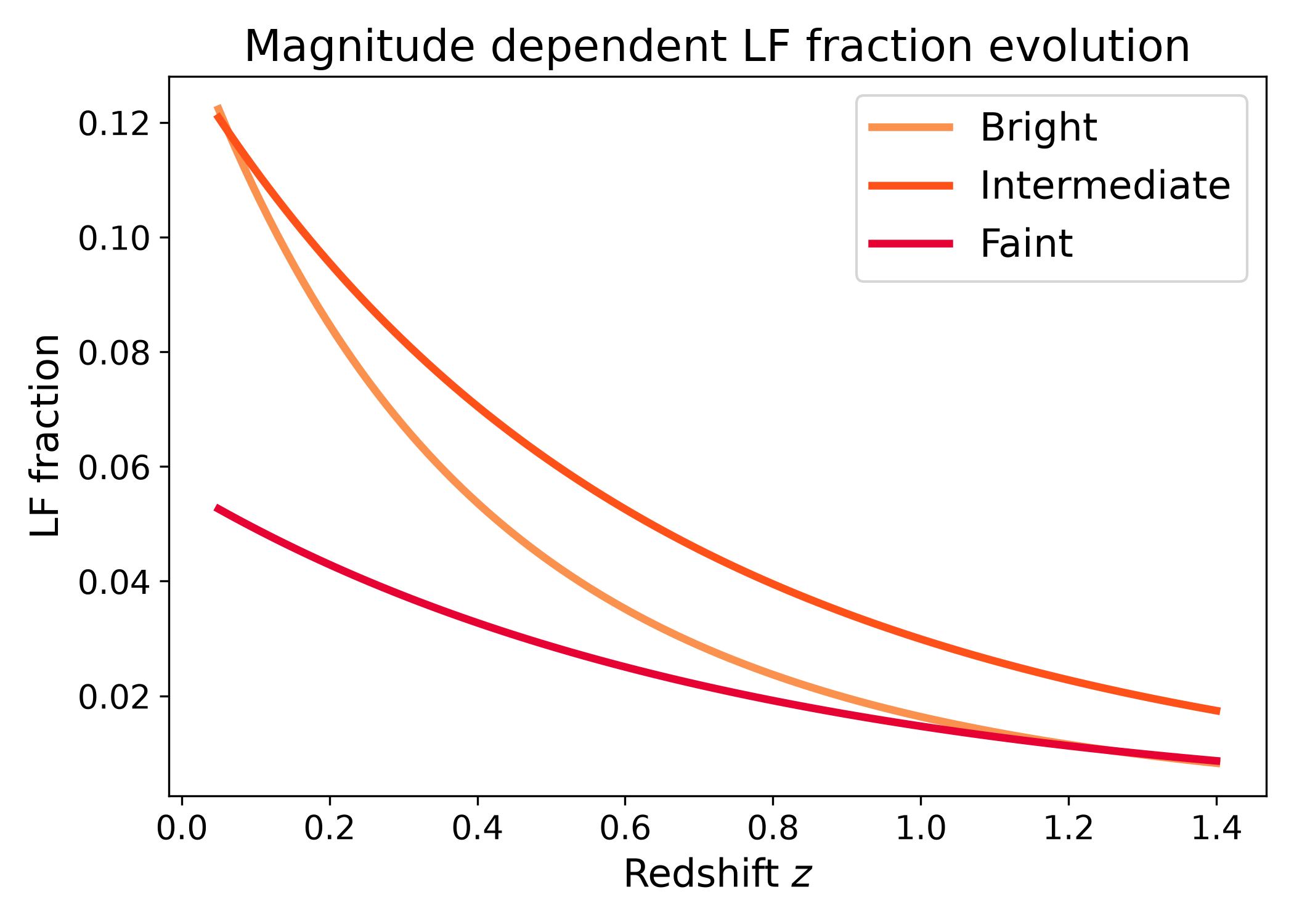
Magnitude range dependence#
Fractions depend on the absolute magnitude range used in the integral. This is useful when comparing bright, intermediate, and faint galaxy selections. In this example both the numerator and denominator luminosity functions evolve with redshift, so the fraction changes with redshift as well as with magnitude range.
Different magnitude ranges can give different population fractions because the relative shape of the numerator and denominator luminosity functions is not constant with magnitude. This plot is useful for checking whether a population fraction is driven mostly by bright galaxies, faint galaxies, or the full selected magnitude interval.
import numpy as np
import matplotlib.pyplot as plt
import cmasher as cmr

from lfkit import LuminosityFunction

LABEL_SIZE = 15
TICK_SIZE = 13
TITLE_SIZE = 17
LEGEND_SIZE = 15

red_lf = LuminosityFunction.evolving_schechter(
    phi_model="linear_p",
    phi_kwargs={"phi_0_star": 3.5e-4, "p": -0.6},
    m_star_model="linear_q",
    m_star_kwargs={"m_0_star": -20.2, "q": 0.2, "z_ref": 0.1},
    alpha_model="constant",
    alpha_kwargs={"alpha": -0.6},
)

all_lf = LuminosityFunction.evolving_schechter(
    phi_model="linear_p",
    phi_kwargs={"phi_0_star": 1.4e-3, "p": 0.5},
    m_star_model="linear_q",
    m_star_kwargs={"m_0_star": -20.8, "q": 1.0, "z_ref": 0.1},
    alpha_model="constant",
    alpha_kwargs={"alpha": -1.25},
)

redshift = np.linspace(0.05, 1.4, 120)

magnitude_windows = [
    (-24.0, -21.0, "Bright"),
    (-21.0, -19.0, "Intermediate"),
    (-19.0, -17.0, "Faint"),
]

colors = cmr.take_cmap_colors("cmr.guppy", 3, cmap_range=(0.0, 0.2))

fig, ax = plt.subplots(figsize=(7.0, 5.0))

for (m_bright, m_faint, label), color in zip(
    magnitude_windows,
    colors,
    strict=True,
):
    fraction = np.array(
        [
            red_lf.fractions.fraction(
                z,
                all_lf,
                m_bright=m_bright,
                m_faint=m_faint,
                n_m=600,
            )
            for z in redshift
        ]
    )

    ax.plot(
        redshift,
        fraction,
        lw=3,
        color=color,
        label=label,
    )

ax.set_xlabel("Redshift $z$", fontsize=LABEL_SIZE)
ax.set_ylabel("LF fraction", fontsize=LABEL_SIZE)
ax.set_title("Magnitude dependent LF fraction evolution", fontsize=TITLE_SIZE)
ax.tick_params(axis="both", labelsize=TICK_SIZE)
ax.legend(frameon=True, fontsize=LEGEND_SIZE, loc="best")
plt.tight_layout()
(png)

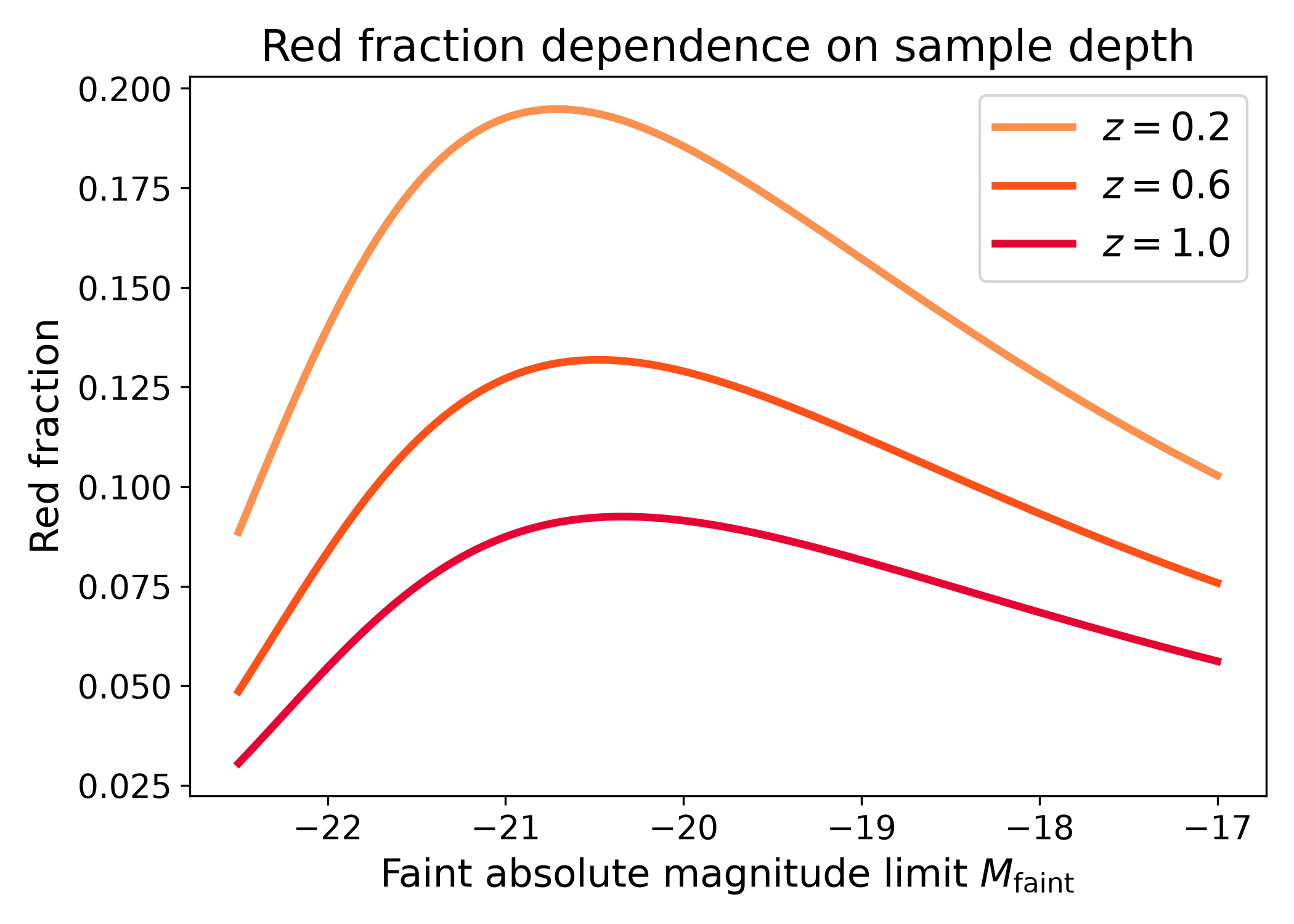
Fraction as a function of faint magnitude limit#
The fraction can also be evaluated as a function of the faint absolute magnitude limit at fixed redshift. This is useful for checking how strongly a population fraction depends on sample depth.
In this example, the bright limit is held fixed while the faint limit is varied.
Moving to fainter magnitude limits adds fainter galaxies to both the numerator
and denominator integrals. If the curves change strongly with M_faint, then
the inferred population fraction is sensitive to the survey depth or luminosity
cut. If the curves are nearly flat, then the fraction is mostly set by the bright
part of the luminosity functions over the plotted magnitude range.
import numpy as np
import matplotlib.pyplot as plt
import cmasher as cmr

from lfkit import LuminosityFunction

LABEL_SIZE = 15
TICK_SIZE = 13
TITLE_SIZE = 17
LEGEND_SIZE = 15

red_lf = LuminosityFunction.evolving_schechter(
    phi_model="linear_p",
    phi_kwargs={"phi_0_star": 4.0e-4, "p": -0.3},
    m_star_model="linear_q",
    m_star_kwargs={"m_0_star": -20.4, "q": 0.4, "z_ref": 0.1},
    alpha_model="constant",
    alpha_kwargs={"alpha": -0.7},
)

all_lf = LuminosityFunction.evolving_schechter(
    phi_model="linear_p",
    phi_kwargs={"phi_0_star": 1.4e-3, "p": 0.3},
    m_star_model="linear_q",
    m_star_kwargs={"m_0_star": -20.7, "q": 0.7, "z_ref": 0.1},
    alpha_model="constant",
    alpha_kwargs={"alpha": -1.2},
)

faint_limits = np.linspace(-22.5, -17.0, 120)
redshifts = [0.2, 0.6, 1.0]

colors = cmr.take_cmap_colors("cmr.guppy", 3, cmap_range=(0.0, 0.2))

fig, ax = plt.subplots(figsize=(7.0, 5.0))

for z, color in zip(redshifts, colors, strict=True):
    fraction = np.array(
        [
            red_lf.fractions.red_fraction(
                z,
                all_lf,
                m_bright=-24.0,
                m_faint=m_faint,
                n_m=600,
            )
            for m_faint in faint_limits
        ]
    )

    ax.plot(
        faint_limits,
        fraction,
        lw=3,
        color=color,
        label=rf"$z={z}$",
    )

ax.set_xlabel(r"Faint absolute magnitude limit $M_{\rm faint}$", fontsize=LABEL_SIZE)
ax.set_ylabel("Red fraction", fontsize=LABEL_SIZE)
ax.set_title("Red fraction dependence on sample depth", fontsize=TITLE_SIZE)
ax.tick_params(axis="both", labelsize=TICK_SIZE)
ax.legend(frameon=True, fontsize=LEGEND_SIZE, loc="best")
plt.tight_layout()
(png)

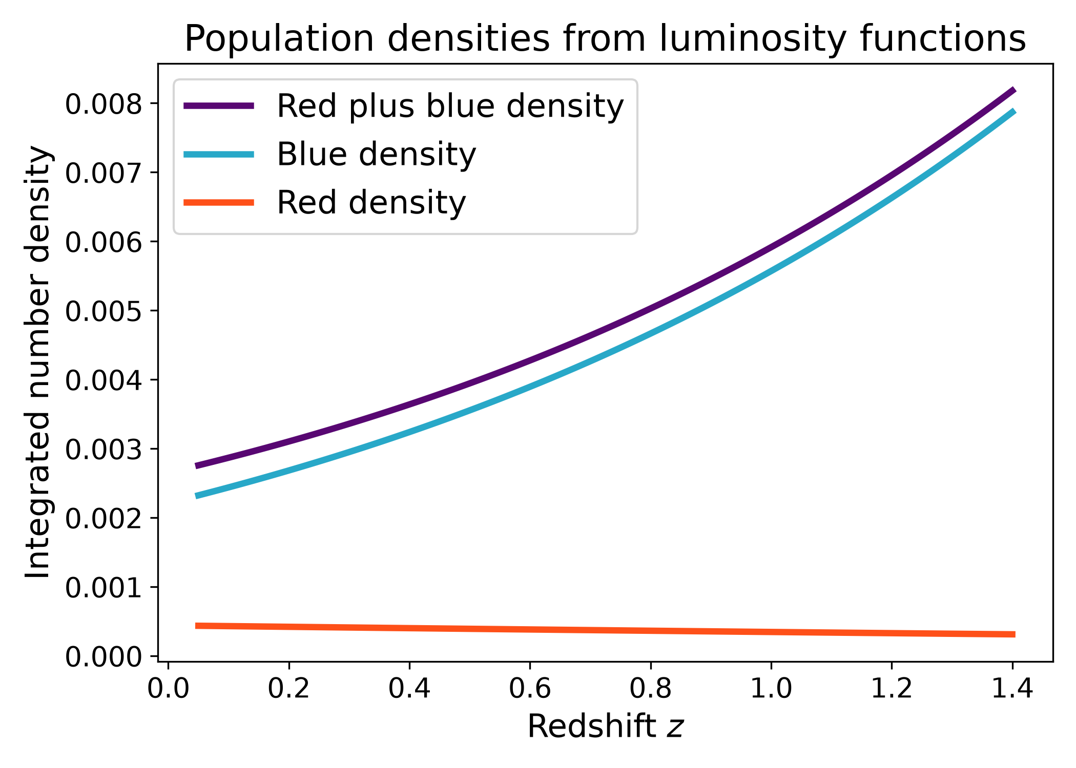
Population densities#
The population_densities helper returns the integrated number densities for
two luminosity functions and their sum. This is useful for checking whether two
subpopulations reconstruct the total population over the chosen magnitude range.
Unlike the fraction helpers, this function returns the integrated densities themselves rather than their ratio. This makes it useful for diagnostics: one can check whether the red and blue densities have sensible amplitudes, whether their sum evolves smoothly, and whether the assumed subpopulation luminosity functions are consistent with the expected total abundance.
import numpy as np
import matplotlib.pyplot as plt
import cmasher as cmr

from lfkit import LuminosityFunction

LABEL_SIZE = 15
TICK_SIZE = 13
TITLE_SIZE = 17
LEGEND_SIZE = 15

red_lf = LuminosityFunction.evolving_schechter(
    phi_model="linear_p",
    phi_kwargs={"phi_0_star": 3.5e-4, "p": -0.4},
    m_star_model="linear_q",
    m_star_kwargs={"m_0_star": -20.3, "q": 0.4, "z_ref": 0.1},
    alpha_model="constant",
    alpha_kwargs={"alpha": -0.7},
)

blue_lf = LuminosityFunction.evolving_schechter(
    phi_model="linear_p",
    phi_kwargs={"phi_0_star": 8.0e-4, "p": 0.5},
    m_star_model="linear_q",
    m_star_kwargs={"m_0_star": -20.8, "q": 0.9, "z_ref": 0.1},
    alpha_model="constant",
    alpha_kwargs={"alpha": -1.25},
)

redshift = np.linspace(0.05, 1.4, 120)

red_density = []
blue_density = []
total_density = []

for z in redshift:
    red_n, blue_n, total_n = red_lf.fractions.population_densities(
        z,
        blue_lf,
        m_bright=-24.0,
        m_faint=-18.0,
        n_m=600,
    )

    red_density.append(red_n)
    blue_density.append(blue_n)
    total_density.append(total_n)

red_density = np.asarray(red_density)
blue_density = np.asarray(blue_density)
total_density = np.asarray(total_density)

red = cmr.take_cmap_colors("cmr.guppy", 3, cmap_range=(0.0, 0.2))[1]
blue = cmr.take_cmap_colors("cmr.guppy", 3, cmap_range=(0.8, 1.0))[1]
total = cmr.take_cmap_colors("cmr.guppy", 3, cmap_range=(0.2, 0.8))[1]

fig, ax = plt.subplots(figsize=(7.0, 5.0))
ax.plot(
    redshift,
    total_density,
    lw=3,
    color=total,
    label="Red plus blue density",
)
ax.plot(
    redshift,
    blue_density,
    lw=3,
    color=blue,
    label="Blue density",
)
ax.plot(
    redshift,
    red_density,
    lw=3,
    color=red,
    label="Red density",
)

ax.set_xlabel("Redshift $z$", fontsize=LABEL_SIZE)
ax.set_ylabel(r"Integrated number density", fontsize=LABEL_SIZE)
ax.set_title("Population densities from luminosity functions", fontsize=TITLE_SIZE)
ax.tick_params(axis="both", labelsize=TICK_SIZE)
ax.legend(frameon=True, fontsize=LEGEND_SIZE, loc="best")
plt.tight_layout()
(png)
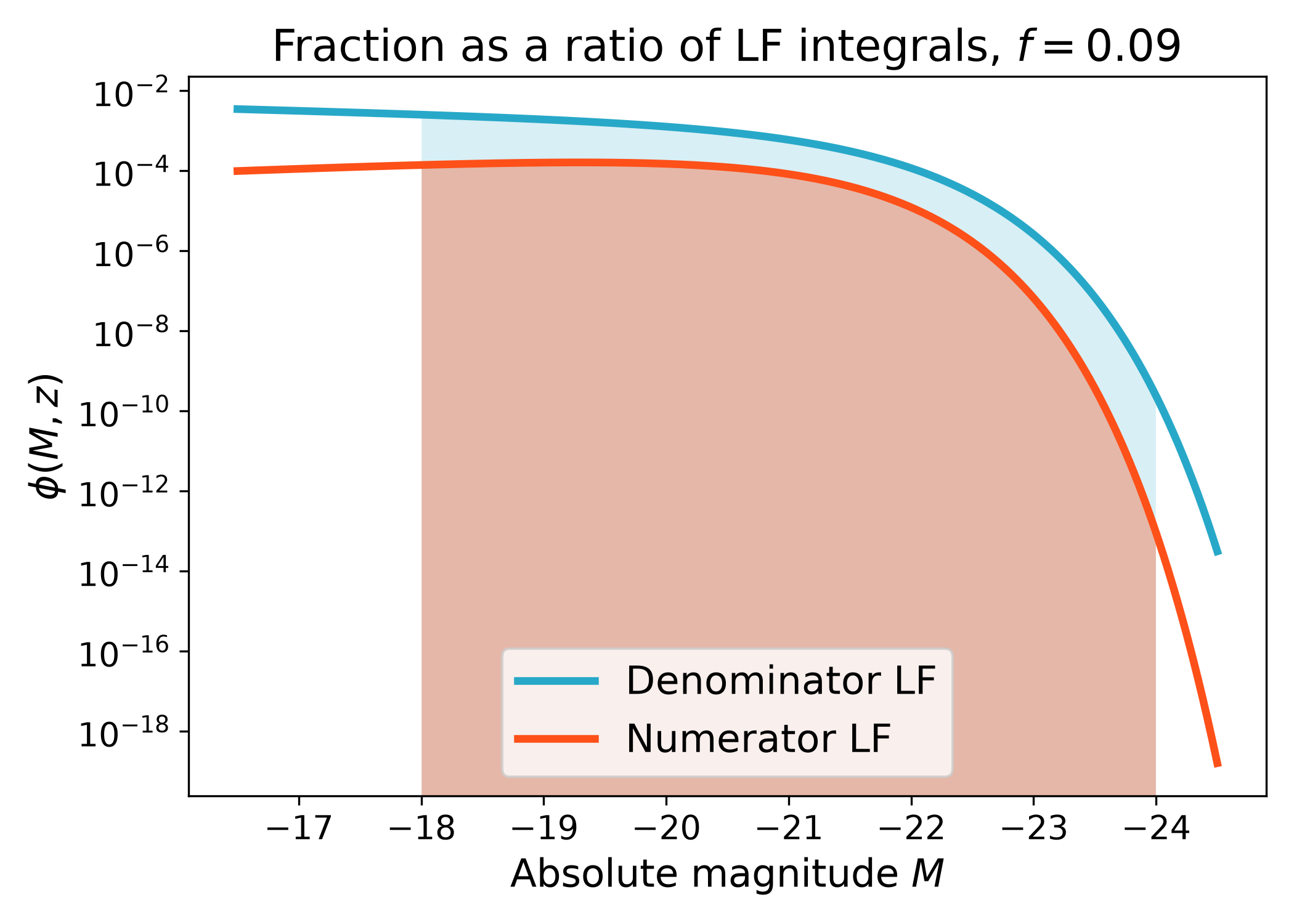
Numerator and denominator integrals#
The fraction is the ratio of two luminosity function integrals over the same
absolute magnitude range. The numerator is the bound luminosity function and the
denominator is the luminosity function passed to fraction.
This diagnostic plot shows the two luminosity functions before integration. The shaded region marks the magnitude range used in the fraction calculation. It is often helpful to inspect this plot when a fraction looks surprising, because the answer may be driven by the relative normalization, faint end slope, or the chosen magnitude limits.
import numpy as np
import matplotlib.pyplot as plt
import cmasher as cmr

from lfkit import LuminosityFunction

LABEL_SIZE = 15
TICK_SIZE = 13
TITLE_SIZE = 17
LEGEND_SIZE = 15

red_lf = LuminosityFunction.evolving_schechter(
    phi_model="linear_p",
    phi_kwargs={"phi_0_star": 4.0e-4, "p": -0.3},
    m_star_model="linear_q",
    m_star_kwargs={"m_0_star": -20.4, "q": 0.4, "z_ref": 0.1},
    alpha_model="constant",
    alpha_kwargs={"alpha": -0.7},
)

all_lf = LuminosityFunction.evolving_schechter(
    phi_model="linear_p",
    phi_kwargs={"phi_0_star": 1.4e-3, "p": 0.3},
    m_star_model="linear_q",
    m_star_kwargs={"m_0_star": -20.7, "q": 0.7, "z_ref": 0.1},
    alpha_model="constant",
    alpha_kwargs={"alpha": -1.2},
)

z = 0.6
absolute_mag = np.linspace(-24.5, -16.5, 400)
m_bright = -24.0
m_faint = -18.0

red_phi = red_lf.phi(absolute_mag, z=z)
all_phi = all_lf.phi(absolute_mag, z=z)

mask = (absolute_mag >= m_bright) & (absolute_mag <= m_faint)

red = cmr.take_cmap_colors("cmr.guppy", 3, cmap_range=(0.0, 0.2))[1]
blue = cmr.take_cmap_colors("cmr.guppy", 3, cmap_range=(0.8, 1.0))[1]

fig, ax = plt.subplots(figsize=(7.0, 5.0))
ax.plot(
    absolute_mag,
    all_phi,
    lw=3,
    color=blue,
    label="Denominator LF",
)
ax.plot(
    absolute_mag,
    red_phi,
    lw=3,
    color=red,
    label="Numerator LF",
)

ax.fill_between(
    absolute_mag[mask],
    0.0,
    all_phi[mask],
    color=blue,
    alpha=0.18,
    linewidth=0.0,
)
ax.fill_between(
    absolute_mag[mask],
    0.0,
    red_phi[mask],
    color=red,
    alpha=0.35,
    linewidth=0.0,
)

fraction = red_lf.fractions.red_fraction(
    z,
    all_lf,
    m_bright=m_bright,
    m_faint=m_faint,
    n_m=800,
)

ax.set_xlabel(r"Absolute magnitude $M$", fontsize=LABEL_SIZE)
ax.set_ylabel(r"$\phi(M, z)$", fontsize=LABEL_SIZE)
ax.set_title(rf"Fraction as a ratio of LF integrals, $f={fraction:.2f}$", fontsize=TITLE_SIZE)
ax.tick_params(axis="both", labelsize=TICK_SIZE)
ax.set_yscale("log")
ax.invert_xaxis()
ax.legend(frameon=True, fontsize=LEGEND_SIZE, loc="best")
plt.tight_layout()
(png)
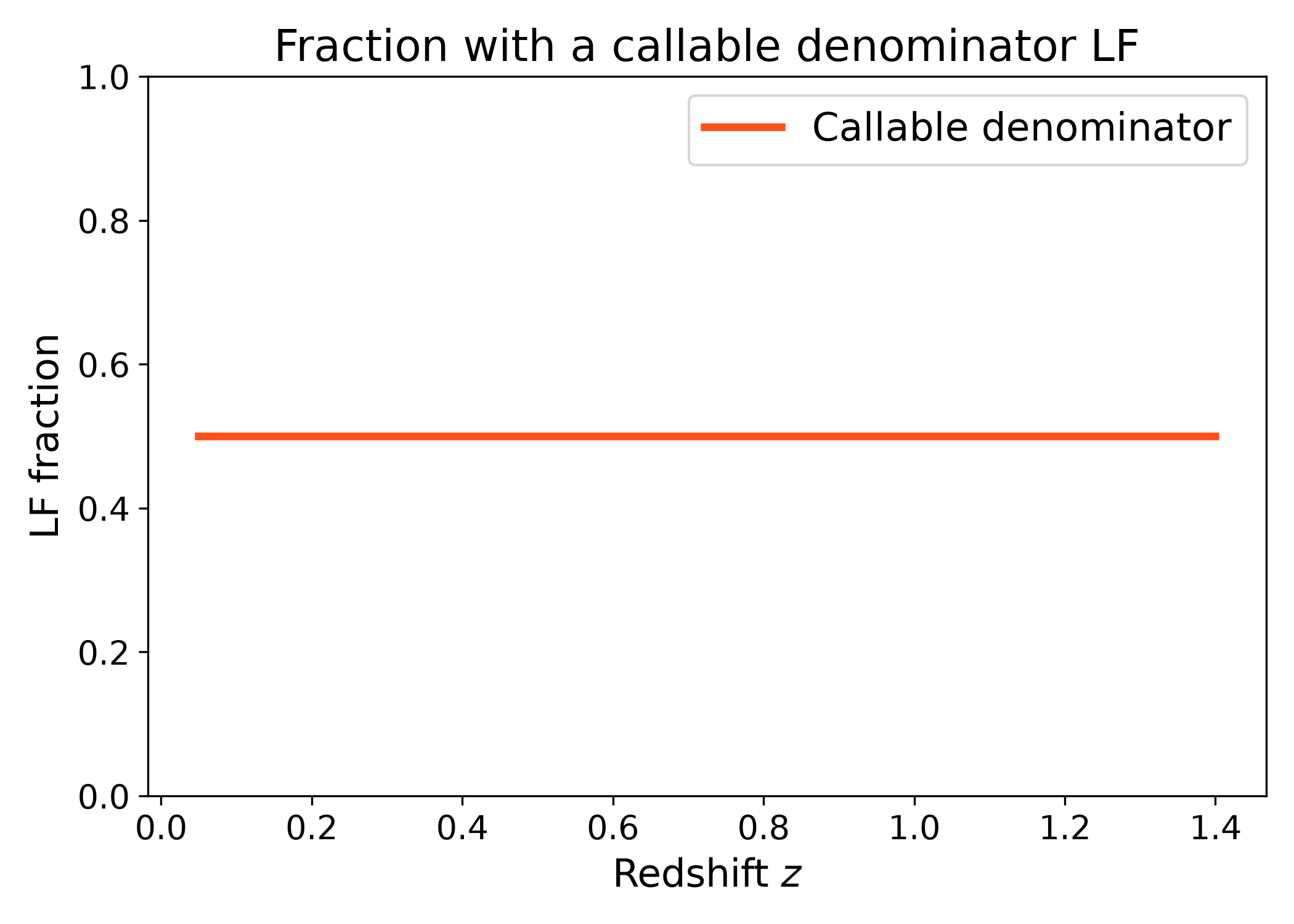
Callable denominator luminosity function#
The denominator can also be any callable with signature
denominator_lf(absolute_mag, redshift). This is useful when the total
luminosity function is produced by a custom model, interpolation, or simulation
output.
This makes the fraction API flexible: the numerator can be an LFKit
LuminosityFunction while the denominator can come from external data or a
user defined model. The only requirement is that the callable returns the
denominator luminosity function evaluated at the requested absolute magnitudes
and redshift.
import numpy as np
import matplotlib.pyplot as plt
import cmasher as cmr

from lfkit import LuminosityFunction

LABEL_SIZE = 15
TICK_SIZE = 13
TITLE_SIZE = 17
LEGEND_SIZE = 15

red_lf = LuminosityFunction.saunders(
    phi_star=6.0e-4,
    m_star=-20.4,
    alpha=-0.9,
    sigma=0.6,
)

def all_lf(absolute_mag, redshift):
    return 2.0 * red_lf.phi(absolute_mag, z=redshift)

redshift = np.linspace(0.05, 1.4, 120)

red_fraction = np.array(
    [
        red_lf.fractions.fraction(
            z,
            all_lf,
            m_bright=-24.0,
            m_faint=-18.0,
            n_m=600,
        )
        for z in redshift
    ]
)

red = cmr.take_cmap_colors("cmr.guppy", 3, cmap_range=(0.0, 0.2))[1]

fig, ax = plt.subplots(figsize=(7.0, 5.0))
ax.plot(
    redshift,
    red_fraction,
    lw=3,
    color=red,
    label="Callable denominator",
)

ax.set_xlabel("Redshift $z$", fontsize=LABEL_SIZE)
ax.set_ylabel("LF fraction", fontsize=LABEL_SIZE)
ax.set_title("Fraction with a callable denominator LF", fontsize=TITLE_SIZE)
ax.tick_params(axis="both", labelsize=TICK_SIZE)
ax.set_ylim(0.0, 1.0)
ax.legend(frameon=True, fontsize=LEGEND_SIZE, loc="best")
plt.tight_layout()
(png)
Note
Fractions are computed from integrated luminosity functions. They are therefore sensitive to the absolute magnitude limits, the LF model choice, and the redshift dependence of both the numerator and denominator models. The denominator luminosity function should represent the full population corresponding to the numerator sample. If this is not true, the returned value is still a ratio of integrals, but it should not be interpreted as a physical population fraction.
The red and blue examples on this page are intended as simple cosmology motivated examples. They should not be interpreted as a complete physical classification of galaxy morphology or evolution.