 Power-law models#
Power-law models describe luminosity functions whose abundance changes as a power of luminosity ratio \(L/L_*\). They are useful for simple scaling tests, bright-end or faint-end approximations, and populations that do not need a Schechter-like exponential cutoff.
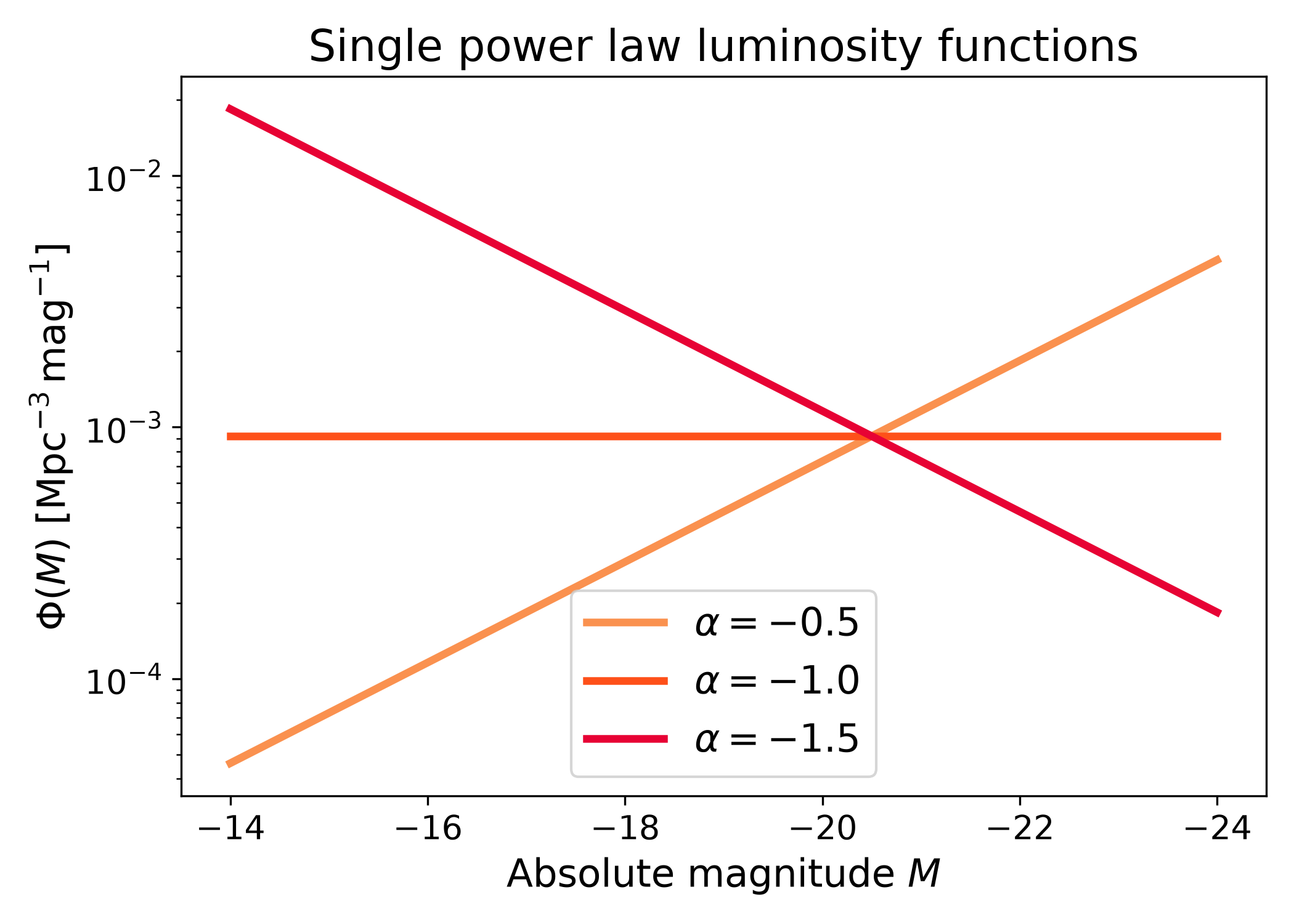
Single power law#
The single power law model has one slope. In magnitude space, this gives a straight-line trend when shown on a logarithmic \(\Phi(M)\) axis.
import numpy as np
import matplotlib.pyplot as plt
import cmasher as cmr

from lfkit import LuminosityFunction

LABEL_SIZE = 15
TICK_SIZE = 13
TITLE_SIZE = 17
LEGEND_SIZE = 15

absolute_mag = np.linspace(-24.0, -14.0, 500)
alphas = [-0.5, -1.0, -1.5]
colors = cmr.take_cmap_colors("cmr.guppy", len(alphas), cmap_range=(0.0, 0.2))

fig, ax = plt.subplots(figsize=(7.0, 5.0))

for alpha, color in zip(alphas, colors):
    lf = LuminosityFunction.power_law(
        phi_star=1.0e-3,
        m_star=-20.5,
        alpha=alpha,
    )
    ax.plot(
        absolute_mag,
        lf.phi(absolute_mag),
        lw=3,
        color=color,
        label=rf"$\alpha={alpha}$",
    )

ax.set_yscale("log")
ax.invert_xaxis()
ax.set_xlabel("Absolute magnitude $M$", fontsize=LABEL_SIZE)
ax.set_ylabel(
    r"$\Phi(M)$ [$\mathrm{Mpc}^{-3}\,\mathrm{mag}^{-1}$]",
    fontsize=LABEL_SIZE,
)
ax.set_title("Single power law luminosity functions", fontsize=TITLE_SIZE)
ax.tick_params(axis="both", labelsize=TICK_SIZE)
ax.legend(frameon=True, fontsize=LEGEND_SIZE, loc="best")
plt.tight_layout()
(png)

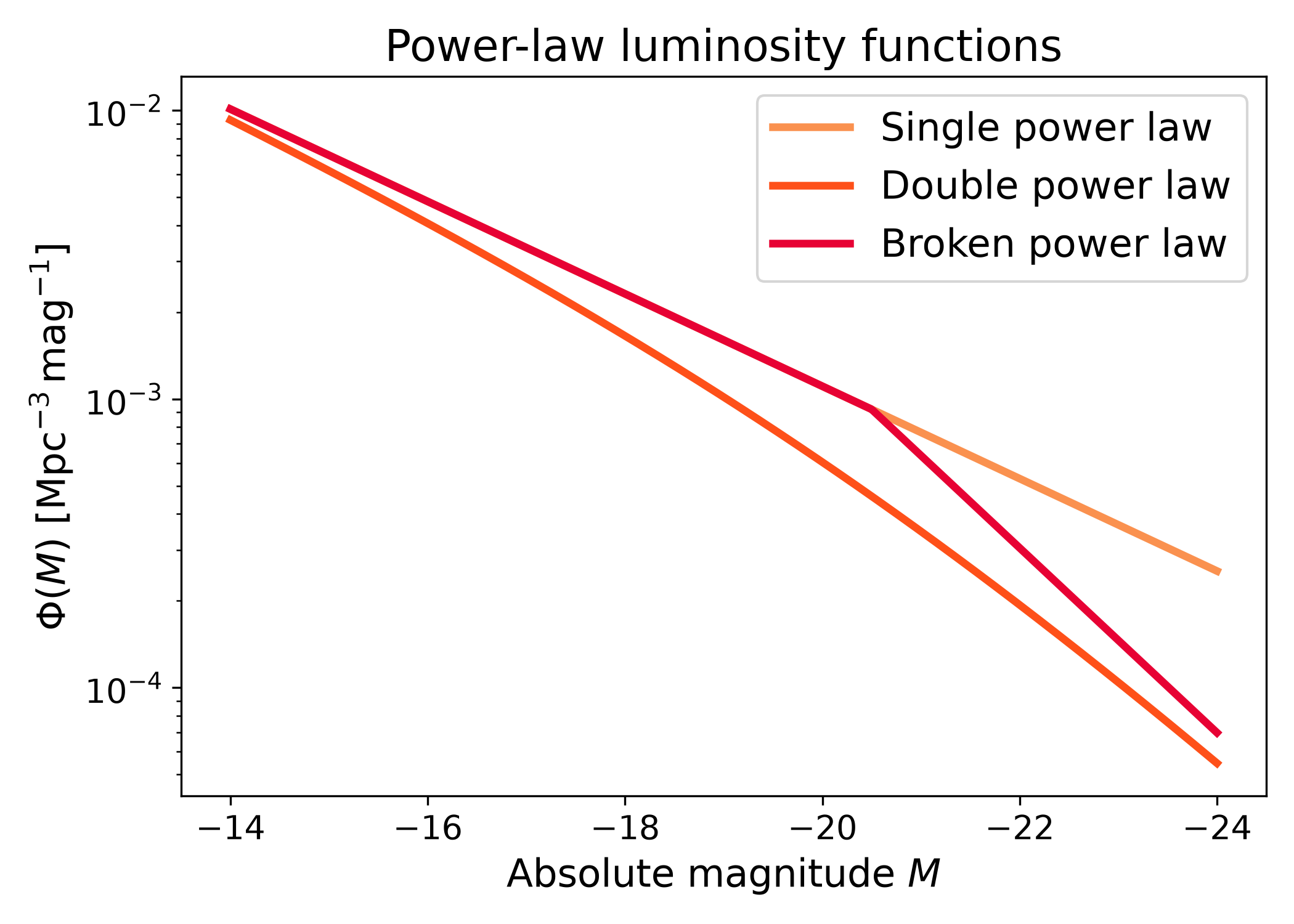
Double and broken power laws#
The double power law smoothly combines two slopes, while the broken power law uses a sharp transition at \(M_*\). These forms are useful when the bright and faint sides need different behaviour without using a Schechter cutoff.
import numpy as np
import matplotlib.pyplot as plt
import cmasher as cmr

from lfkit import LuminosityFunction

LABEL_SIZE = 15
TICK_SIZE = 13
TITLE_SIZE = 17
LEGEND_SIZE = 15

single = LuminosityFunction.power_law(
    phi_star=1.0e-3,
    m_star=-20.5,
    alpha=-1.4,
)

double = LuminosityFunction.double_power_law(
    phi_star=1.0e-3,
    m_star=-20.5,
    alpha=-1.4,
    beta=-1.8,
)

broken = LuminosityFunction.broken_power_law(
    phi_star=1.0e-3,
    m_star=-20.5,
    alpha_faint=-1.4,
    alpha_bright=-1.8,
)

absolute_mag = np.linspace(-24.0, -14.0, 500)
colors = cmr.take_cmap_colors("cmr.guppy", 3, cmap_range=(0.0, 0.2))

fig, ax = plt.subplots(figsize=(7.0, 5.0))
ax.plot(
    absolute_mag,
    single.phi(absolute_mag),
    lw=3,
    color=colors[0],
    label="Single power law",
)
ax.plot(
    absolute_mag,
    double.phi(absolute_mag),
    lw=3,
    color=colors[1],
    label="Double power law",
)
ax.plot(
    absolute_mag,
    broken.phi(absolute_mag),
    lw=3,
    color=colors[2],
    label="Broken power law",
)

ax.set_yscale("log")
ax.invert_xaxis()
ax.set_xlabel("Absolute magnitude $M$", fontsize=LABEL_SIZE)
ax.set_ylabel(
    r"$\Phi(M)$ [$\mathrm{Mpc}^{-3}\,\mathrm{mag}^{-1}$]",
    fontsize=LABEL_SIZE,
)
ax.set_title("Power-law luminosity functions", fontsize=TITLE_SIZE)
ax.tick_params(axis="both", labelsize=TICK_SIZE)
ax.legend(frameon=True, fontsize=LEGEND_SIZE, loc="best")
plt.tight_layout()
(png)
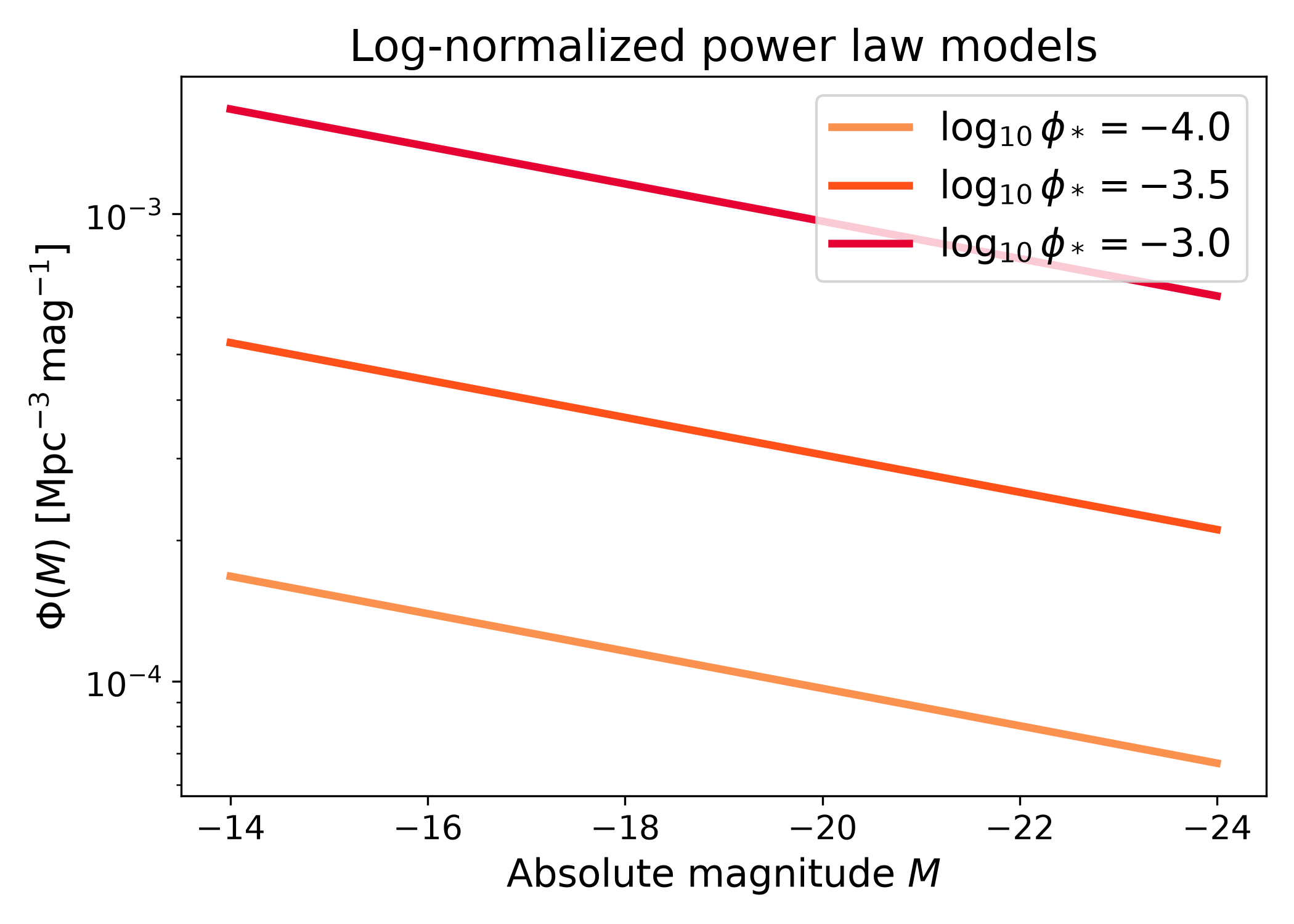
Log-normalized power law#
The log-normalized power law model is the same power law shape, but the
normalization is supplied as log_phi_star. This is convenient for fitting
or sampling applications where the normalization is naturally varied in
logarithmic space.
import numpy as np
import matplotlib.pyplot as plt
import cmasher as cmr

from lfkit import LuminosityFunction

LABEL_SIZE = 15
TICK_SIZE = 13
TITLE_SIZE = 17
LEGEND_SIZE = 15

absolute_mag = np.linspace(-24.0, -14.0, 500)
log_phi_stars = [-4.0, -3.5, -3.0]
colors = cmr.take_cmap_colors(
    "cmr.guppy",
    len(log_phi_stars),
    cmap_range=(0.0, 0.2),
)

fig, ax = plt.subplots(figsize=(7.0, 5.0))

for log_phi_star, color in zip(log_phi_stars, colors):
    lf = LuminosityFunction.log_power_law(
        log_phi_star=log_phi_star,
        m_star=-20.5,
        alpha=-1.1,
    )
    ax.plot(
        absolute_mag,
        lf.phi(absolute_mag),
        lw=3,
        color=color,
        label=rf"$\log_{{10}}\phi_*={log_phi_star}$",
    )

ax.set_yscale("log")
ax.invert_xaxis()
ax.set_xlabel("Absolute magnitude $M$", fontsize=LABEL_SIZE)
ax.set_ylabel(
    r"$\Phi(M)$ [$\mathrm{Mpc}^{-3}\,\mathrm{mag}^{-1}$]",
    fontsize=LABEL_SIZE,
)
ax.set_title("Log-normalized power law models", fontsize=TITLE_SIZE)
ax.tick_params(axis="both", labelsize=TICK_SIZE)
ax.legend(frameon=True, fontsize=LEGEND_SIZE, loc="best")
plt.tight_layout()
(png)